Topic 2 Getting Started With RMarkdown
2.1 What is RMD
R Markdown is a file format for making dynamic documents with R. An R Markdown document is written in markdown (an easy-to-write plain text format) and contains chunks of embedded R code, like the document below.
RMarkdown makes use of Markdown syntax. Markdown is a very simple ‘markup’ language that provides methods for creating documents with headers, images, links, etc. from plain text files while keeping the original plain text file easy to read.
R Markdown files are the source code for rich, reproducible documents. We can transform an R Markdown file in two ways.
knit - The rmarkdown package will call the
knitrpackage.knitrwill run each chunk of R code in the document and append the results of the code to the document next to the code chunk.convert - The rmarkdown package will use the pandoc program to transform the file into a new format such as HTML, PDF, or Microsoft Word file. RMarkdown will preserve the text, code results, and formatting contained in the original.Rmd file.
The term render refers to the above two-step process of knitting and converting an R Markdown file.
2.1.1 Create an RMarkdown file
To create a new RMarkdown file (.Rmd), select File -> New File -> R Markdownin RStudio, then choose one of the file types we want to create.
The newly created.Rmd file comes with an RMarkdown template with basic instructions.
2.1.2 The YAML Header
At the top of any RMarkdown script is a YAML (Yet Another Markup Language) header section enclosed by ---. By default, this includes a title, author, date and the file type you want to output to.
Many other options are available for different functions and formatting, see here for .html options and here for .pdf options. Rules in the header section will alter the whole document.
The following is the simplest YMAL template.
---
title: "Introduction to RMarkdown"
author: "Cheng Peng"
date: "12/25/2021"
output:
  html_document: default
  html_notebook: default
editor_options:
  chunk_output_type: inline
---
Note that YAML is automatically generated that reflects the choice of the file type and related file specifications. Therefore, we don’t need to know YAML unless we want to modify it manually.
2.1.3 Markdown Syntax
- Formatting Text
- Italic - single asterisk -> italic.
- bold - double asterisks -> bold face
code- code in text
Header# Header 1: single#- level 1 header## Header 2: double##- level 2 header### Header 3: triple###- level 3 header
- List
* Unordered list- single asterisk+space -> unordered list1. Ordered list- numbered list
- Hyperlink
< url >- Example: https://www.wcupa.edu/[link-name](url)- Example: WCUPA
- LaTex Equations Syntax
$ LaTex commands $- Example: \(y = \beta_0 + \beta_1 x\)
2.2 Code Chunks
Code that is included in .Rmd document should be enclosed by three backward apostrophes ``` (grave accents!). These are known as code chunks. An executable code chunk looks like the following.
The first line:```{r chunk-name-with-no-spaces} contains the language (r) in this case, and the name of the chunk, and other optional code chunk options. Next to the {r}, there is a chunk name. The chunk name is not necessarily required however, it is good practice to give each chunk a unique name to support more advanced knitting approaches.
If the language is not specified in the curly bracket, the chunk is simply a verbatim environment that keeps the content in the knitted document. For example, the content in the following chunk will not be executed.
The context will not be processed when converting this document to HTML,
PDF, or other document formats.
2.3 Inserting Graphics
There are two different ways to include images into RMD: Generated by the code in the code chunk and external source of images.
- R Generated Graphics
Including R-generated graphics into RMD is straightforward. The following example shows how to embed a graphic with some code chunk options to layout the graphic.
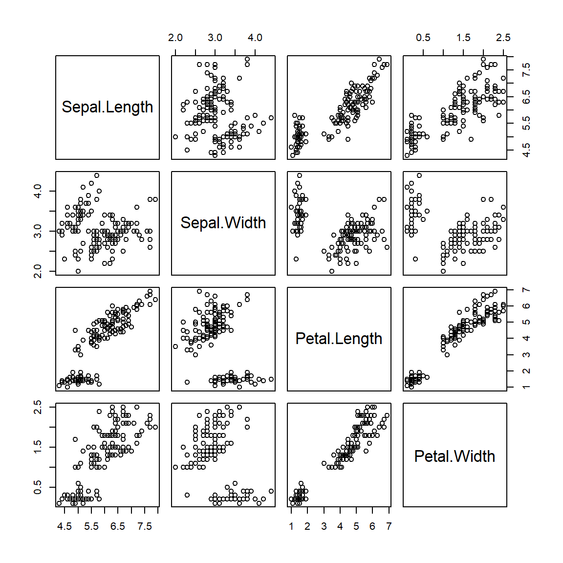
Figure 2.1: Pairwise scatter plot of iris data set
- External Images
There are several ways to include an external image into RMD documents.
- Using HTML
imgTag
<br>
<center><img src="https://github.com/pengdsci/sta553/blob/main/image/boats.jpg?raw=true" alt="Portland Headlight" height="400" width="600"></center>
<br>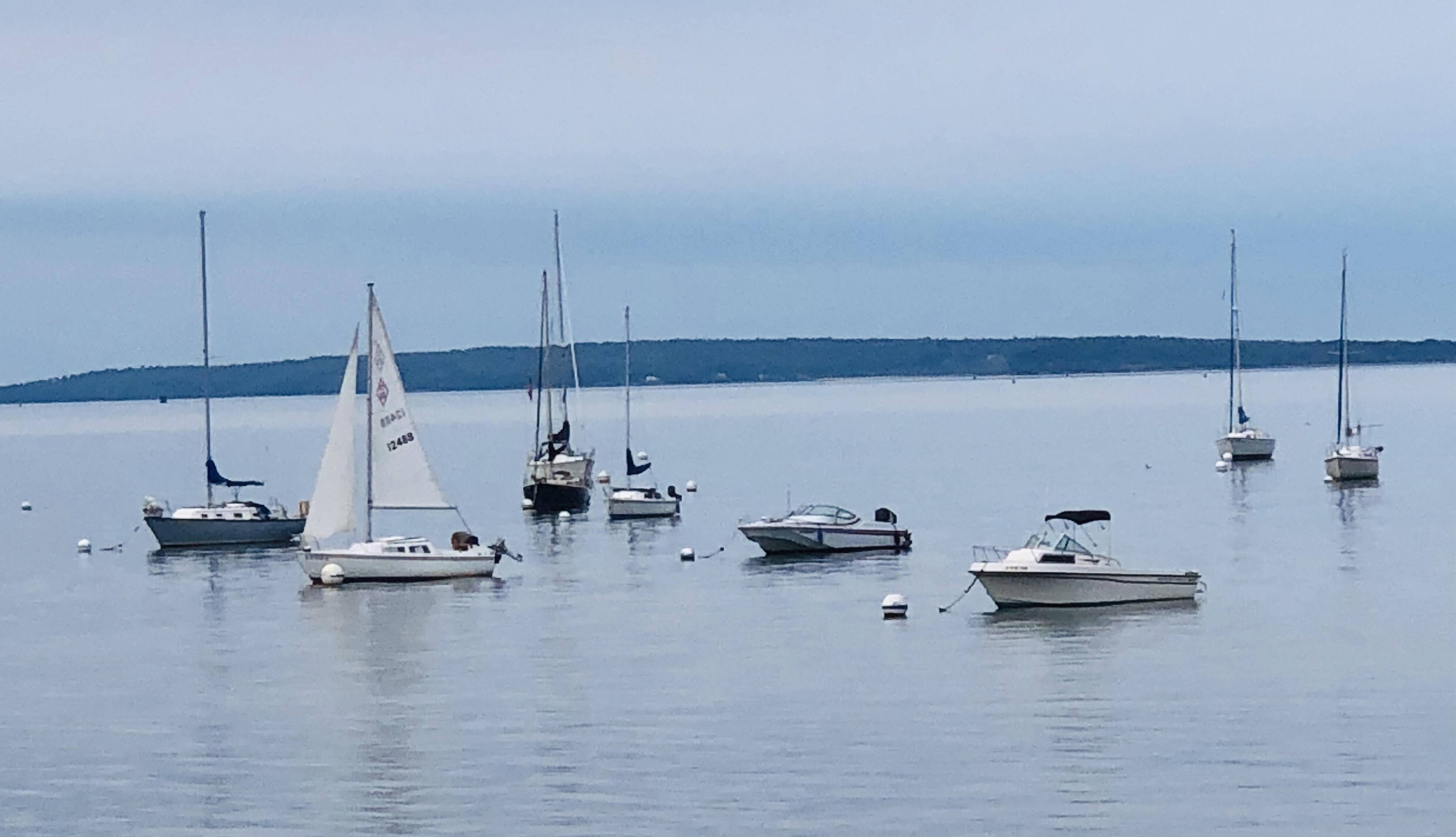
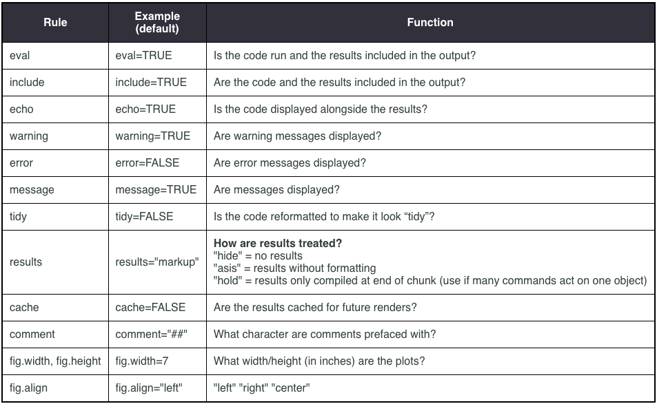
Figure 2.2: RMarkdown Code Chunk Options
- Using
knitrFunction
Chunk options: fig.align='center', echo=FALSE, fig.cap="White Mountain", out.width = '50%'
knitr::include_graphics("img01/w01-WhiteMountain.jpg)
Figure 2.3: White Mountain
2.4 Inserting Tables
A quality table is also an important visualization tool. We introduce three methods for inserting nice-looking tables into the RMD document.
- Extracting R Output Matrix Using
kable()Function
For example, we fit a linear regression model using iris data and extract the statistics of model fit to define a table.
data(iris)
iris.model = lm(Sepal.Length~., data = iris)  # fit a linear model
mod.stats = coef(summary(iris.model))         # inferential stats of coefficients
kable(mod.stats) # | Estimate | Std. Error | t value | Pr(>|t|) | |
|---|---|---|---|---|
| (Intercept) | 2.1712663 | 0.2797942 | 7.760228 | 0.0000000 |
| Sepal.Width | 0.4958889 | 0.0860699 | 5.761466 | 0.0000000 |
| Petal.Length | 0.8292439 | 0.0685276 | 12.100867 | 0.0000000 |
| Petal.Width | -0.3151552 | 0.1511958 | -2.084418 | 0.0388883 |
| Speciesversicolor | -0.7235620 | 0.2401689 | -3.012721 | 0.0030596 |
| Speciesvirginica | -1.0234978 | 0.3337263 | -3.066878 | 0.0025843 |
- Markdown Table
We can manually create a Markdown table. See the following example.
| Plant | Temp. | Growth |
|:------|:-----:|-------:|
| A     | 20    | 0.65   |
| B     | 20    | 0.95   |
| C     | 20    | 0.15   |
The resulting Markdown has the following
| Plant | Temp. | Growth |
|---|---|---|
| A | 20 | 0.65 |
| B | 20 | 0.95 |
| C | 20 | 0.15 |
The Markdown table syntax is explained in the following:
:----:: Centre:-----: Left-----:: Right------: Auto
- HTML Table
<table border = 1>
  <tr>
    <th>Company</th>
    <th>Contact</th>
    <th>Country</th>
  </tr>
  <tr>
    <td>Alfreds Futterkiste</td>
    <td>Maria Anders</td>
    <td>Germany</td>
  </tr>
  <tr>
    <td>Centro comercial Moctezuma</td>
    <td>Francisco Chang</td>
    <td>Mexico</td>
  </tr>
</table>
A basic HTML table
| Company | Contact | Country |
|---|---|---|
| Alfreds Futterkiste | Maria Anders | Germany |
| Centro comercial Moctezuma | Francisco Chang | Mexico |
- LaTex Table
This will not work if we knit the RMD to HTML since it is a LaTex table.
\begin{table}
\centering
\begin{tabular}{llll}
1 & 2 & 3 & 4  \\
1 & 3 & 4 & 6  \\
3 & 4 & 1 & 8  \\
5 & 2 & 0 & 1
\end{tabular}
\end{table}
2.5 Creating PDF
Creating .pdf documents for printing in A4 requires a bit more fiddling around. RStudio uses another document compiling system called LaTeX to make .pdf documents.
The easiest way to use LaTeX is to install the TinyTex distribution from within RStudio. First, restart the R session (Session -> Restart R), then run these lines in the console:
install.packages("tinytex")
tinytex::install_tinytex()
Becoming familiar with LaTeX will give you a lot more options to make your R Markdown .pdf look pretty, as LaTeX commands are mostly compatible with R Markdown, though some googling is often required.
To install a full-functioning LaTex, MikTex is recommended. The official website for MikTex is https://miktex.org/download.
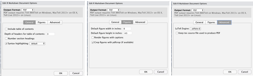
We can also choose different options to make a nicer PDF by clicking the arrow on the gear sign (![]() ) and then selection
) and then selection Output Options.... Then select Output Format: as PDF. Then we can choose appropriate options.
2.6 Miscellaneous
We have introduced the basics of R Markdown. Several good features are worth mentioning.
2.6.1 Markdown Presentations
R Markdown can prepare presentations in HTML slides, PDF Beamer, and Microsoft PowerPoint Presentation. Some of the lecture notes will be prepared in PDF Beamer.
2.6.2 Shiny Apps and RMarkdown
A recent development is the ability to put Shiny elements into an RMarkdown document.
These documents, again, need a Shiny server to run, but take advantage of the easy formatting of RMarkdown to present the user interface - server and UI elements sit in the same document.
- RMarkdown - supplies the HTML instead of a
ui.Rfile. - Shiny - supplied reactive components within your RMarkdown
We will prepare shiny lecture notes using RMarkdown in this class.
2.6.3 Working Directory
Sometimes we may want to use a specific directory as the working directory to store relevant files associated with the same analysis. The usual way to change the working directory is setwd(), but please note that setwd() is not persistent in R Markdown (or other types of knitr source documents), which means setwd() only works for the current code chunk, and the working directory will be restored after this code chunk has been evaluated.
It is not encouraged to use setwd() in RMarkdown documents.
2.6.4 CSS Style
We can include a CSS-style file to format HTML. The style file used in this RMD is given below.
<style type="text/css">
div#TOC li {
    list-style:none;
    background-image:none;
    background-repeat:none;
    background-position:0;
}
h1.title {
  font-size: 24px;
  color: darkRed;
  text-align: center;
}
h4.author { /* Header 4 - and the author and data headers use this too  */
    font-size: 18px;
  font-family: "Times New Roman", Times, serif;
  color: DarkRed;
  text-align: center;
}
h4.date { /* Header 4 - and the author and data headers use this too  */
  font-size: 18px;
  font-family: "Times New Roman", Times, serif;
  color: DarkBlue;
  text-align: center;
}
h1 { /* Header 3 - and the author and data headers use this too  */
    font-size: 22px;
    font-family: "Times New Roman", Times, serif;
    color: darkred;
    text-align: center;
}
h2 { /* Header 3 - and the author and data headers use this too  */
    font-size: 18px;
    font-family: "Times New Roman", Times, serif;
    color: navy;
    text-align: left;
}
h3 { /* Header 3 - and the author and data headers use this too  */
    font-size: 15px;
    font-family: "Times New Roman", Times, serif;
    color: darkred;
    font-face: bold;
    text-align: left;
}
h4 { /* Header 4 - and the author and data headers use this too  */
    font-size: 18px;
    font-family: "Times New Roman", Times, serif;
    color: darkred;
    text-align: left;
}
</style>