Topic 15 Getting Started with R Shiny
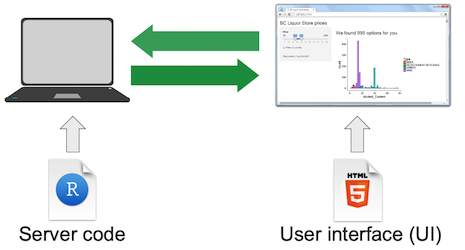
RShiny apps must run on a shiny server. This eBook (all three formats will be stored in the GitHub repository. We will not be able to show the interactivity of apps. Instead, screenshots will be included in this eBook to show the GUI designed based on the code. One can run the provided source code and run it on the local machine and see the interactive effect of the apps.
Shiny is a powerful and flexible R package that makes it easy to build interactive web applications and dynamic dashboards straight from R. These applications can be hosted on a standalone webpage or embedded in R Markdown documents.
Shiny is 10 years old now!
15.1 The IDE of RShiny Apps
Studio IDE has an environment for developing R shiny apps. There are two different ways to write shiny apps code in R:
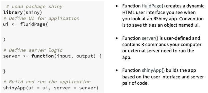
Single File Method: In this single file, we write a ui function to design the UI and a server function to process user input information and output computed information.
Two File Method: In this method consists of two separate files: ui.R for designing UI and server.R for processing and computing the user input information. Both script files must be saved in the same folder you created for this app. If we choose to use this method, R will automatically create the two template files in the designated folder.
15.2 Embedding Shiny Apps in RMarkdown
We can also write shiny apps in RMarkdown. This is convenient and useful for drafting analysis reports that contain shiny apps and other interactive plots. This note is prepared to illustrate how to develop shiny apps with numerous examples. When writing shiny apps in RMarkdown, we have to specify runtime: shiny in the YAML header in order to correctly render the apps.
15.3 Components of An Shiny Applications
Programmatically, a Shiny application is simply a directory containing an R script called app.R which is made up of a user interface (ui) object and a server function. This folder could also contain some additional data, scripts, or other resources required to support the application.
15.4 The Anatomy of a Shiny Application
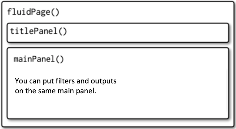
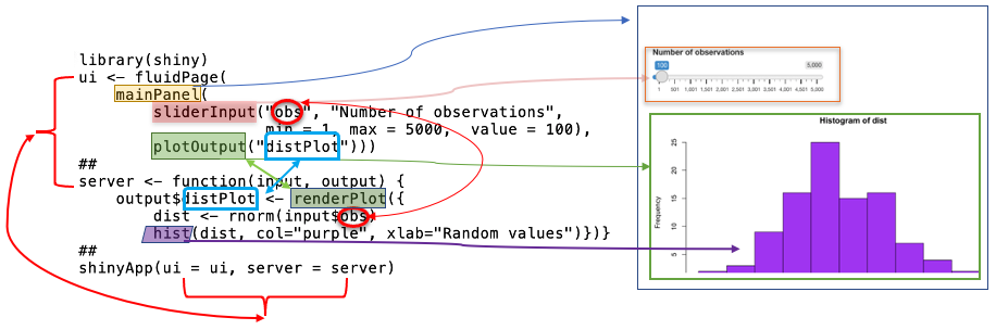
The following example shiny app uses a single panel layout. It simply stacks all informational panels on the same fluidPage (graphical page). We use the layout as an example to illustrate the structure of the R shiny app and use it to develop the first R shiny app for this class.
uidesigns the layout of the app usesmainPanel(). There are many different layout designs to be discussed later.sliderInputdesigns the slider input widget.server()contains all R code that generates the output.
library(shiny)
### global R code
###
### if you have R functions that are used repeatedly or the
### The function itself is sophisticated, you can put it here
### to make your code tidy
##
##
### user interface - layout web interface for input and outputs
###
ui <- fluidPage(
    mainPanel(                                            # main panel, in general, we could add
                                                          # a sidePanel for inputs
        sliderInput(inputId = "obs",                      # sliderInput - one of the input widgets
                                                          # 'obs' = input parameter via the slider
                      label = "Number of observations",   # The title of the slider
                        min = 1,                          # the minimum input value
                        max = 5000,                       # the maximum input value
                      value = 100),                       # the default input is set to be 100

        plotOutput(outputId = "distPlot")         # a place holder for the output to be
                                                  # created inside the server function.
                                                  # "distPlot" is the reference of the plot output.
    )
)
#######
####### information to be processed and computed from the server side.
####### All code we wrote for visualization can be placed inside the server function as needed.
#######
server <- function(input, output) {    # sever function passes two parameters:
                                       # 'input' = value from UI's sliderInput "obs",
                                       # 'output' = 'disPlot' in the output place holder.
    output$distPlot <- renderPlot({    # 'renderPlot' prepares output plot - pay attention to the reference function.
                                       # This is how we pass the input information to the server
                                       # and render the computed information to display in the output panel.
        dist <- rnorm(input$obs)       # simulate standard normal random numbers
                                       #  'obs' = from sliderInput in the UI
        hist(dist,                     # make a histogram use the regular plot function hist()
            col="purple",              # fill the vertical bar with a color
            xlab="Standard Normal Random Numbers ",       # add a horizontal label
            main = paste("Sample Size:", input$obs)
            )
    })
}
### link the ui and server functions
shinyApp(ui = ui, server = server) 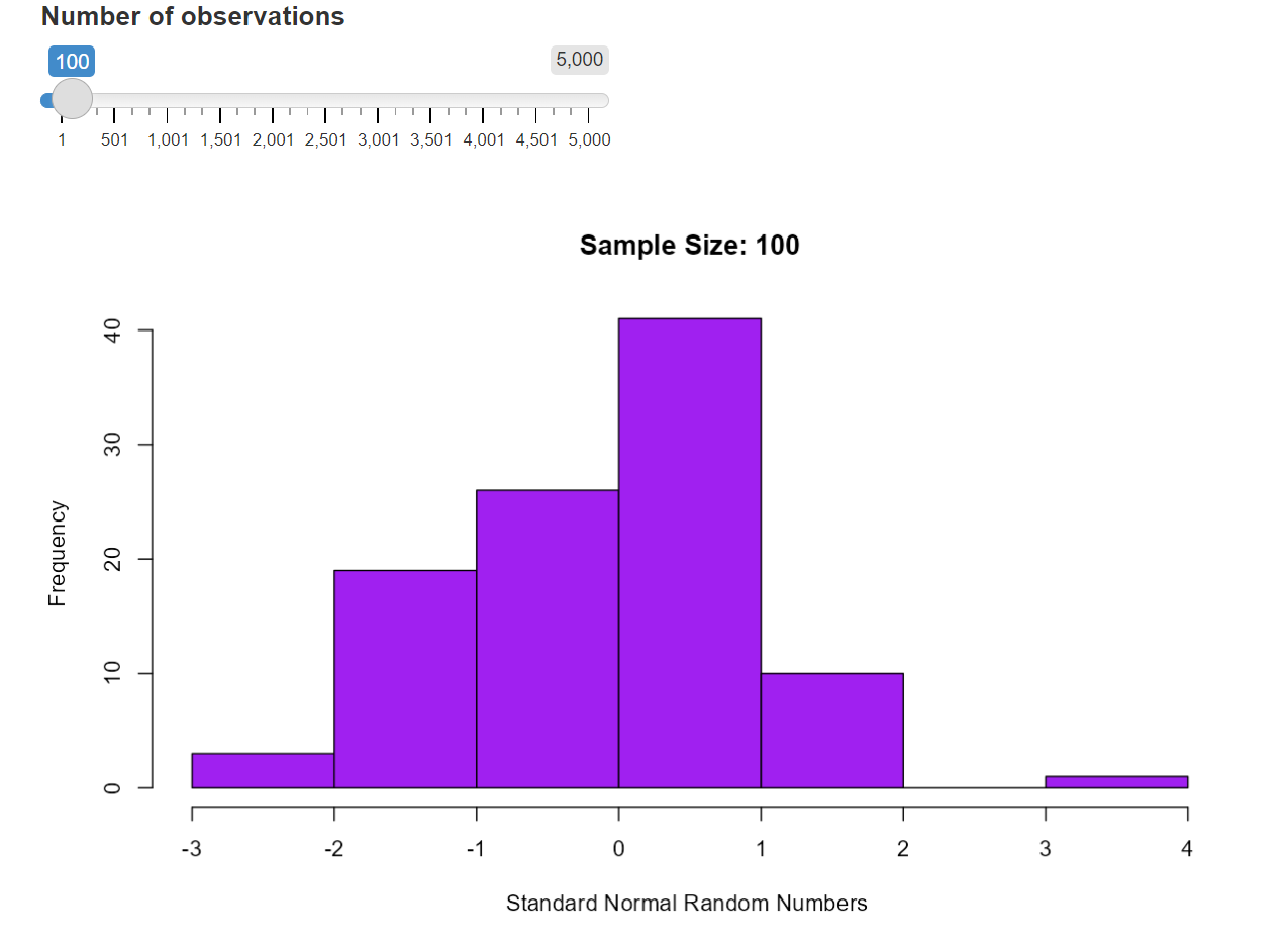
15.6 Some Built-in Demonstrations of Shiny Apps
Package Shiny comes with some example apps. Enter any of the following in the R Console to see the Shiny app in action along with the code. The built-in shiny apps are named using their corresponding input widget names.
We modified the function and renamed it as runExample2 to call apps without showing the source R code. If you only want to see the siderbarPanel and the mainePanel, you simply use the function runExample(). The source code of the modified function is not included in this class note. If you are interested in looking at the code, use the hyperlink in the following code chunk to view it.
source("https://raw.githubusercontent.com/pengdsci/sta553/main/shiny/shinyCodeExtractor.txt")
#runExample2("01_hello")        # a histogram
#runExample("02_text")         # tables and data frames
#runExample("03_reactivity")   # a reactive expression
#runExample("04_mpg")          # global variables
#runExample("05_sliders")      # slider bars
#runExample("06_tabsets")      # tabbed panels
#runExample("07_widgets")      # help text and submit buttons
#runExample("08_html")         # Shiny app built from HTML
#runExample("09_upload")       # file upload wizard
#runExample("10_download")     # file download wizard
#runExample("11_timer")        # an automated timer
15.7 UI Layout Designs - A Glance
The UI function is responsible for designing the user interface design that includes the layout of the application and placeholders for the desired outputs.
15.7.1 Siderbar Layout
The basic shiny app side bar layout has the following structure.
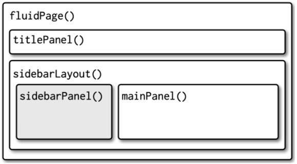
The UI function should look like
ui = fluidPage(
        titlePanel(),
        sidebarLayout(
           sidebarPanel(),
           mainPanel()
        )
     )
For example, we can modify the above code to create an app with a sidebar navigation panel and an output main panel.
library(shiny)
### global R code
###
### if you have R functions that are used repeatedly or the
### the function itself is sophisticated, you can put it here
### to make your code tidy
##
##
### user interface - layout web interface for input and outputs
###
ui <- fluidPage(
    ##  overall title of  the app
    titlePanel("Distribution of A Random Variable"),      # title of the shiny app
    ## side bar navigation panel
    sidebarPanel(                                         # a sidePanel for inputs
        sliderInput(inputId = "obs",                      # sliderInput - one of the input widgets
                                                          # 'obs' = input parameter via the slider
                      label = "Number of observations",   # The title of the slider
                        min = 1,                          # the minimum input value
                        max = 5000,                       # the maximum input value
                      value = 100),                       # the default input is set to be 100

    ),

    mainPanel(                                    # main panel, in general, we could add
        plotOutput(outputId = "distPlot")         # a place holder for the output to be
                                                  # created inside the server function.
                                                  # "distPlot" is the reference of the plot output.
    )
)
#######
####### information to be processed and computed from server side.
####### all code we wrote for visualization can place inside the server function as needed.
#######
server <- function(input, output) {    # sever function passes two parameters:
                                       # 'input' = value from UI's sliderInput "obs",
                                       # 'output' = 'disPlot' in the output place holder.
    output$distPlot <- renderPlot({    # 'renderPlot' prepares output plot - pay attention to the reference function.
                                       # this how you pass the input information to the server
                                       # and render the computed information to display in the output panel.
        dist <- rnorm(input$obs)       # simulate standard normal random numbers
                                       #  'obs' = from sliderInput in the UI
        hist(dist,                     # make a histogram use the regular plot function hist()
            col="purple",              # fill the vertical bar with a color
            xlab="Random values")      # add horizontal label
    })
}
### link the ui and server functions
shinyApp(ui = ui, server = server) 
In some situations, we more complex UI may be necessary, UI function can define a more sophisticated layout. For example, we can consider multi-row UI design such as the following layout.
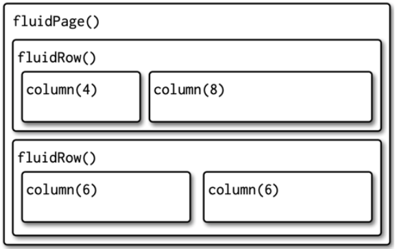
Each row is made up of 12 columns and the first argument to column() gives how many of those columns to occupy. We will illustrate how to develop shiny apps using this layout later.
15.8 Some Basic Input Widgets
The 11 built-in apps in the demonstration have provided different forms of input methods. Here are some that are used frequently in practice. We have used sliderInput in the example. Next, we list a few more commonly used ones.
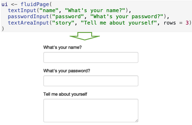
15.8.1 Free Text
This input method is practically useful when building apps that take information from the user directly for analysis and visualization. The following UI design is a general text input.
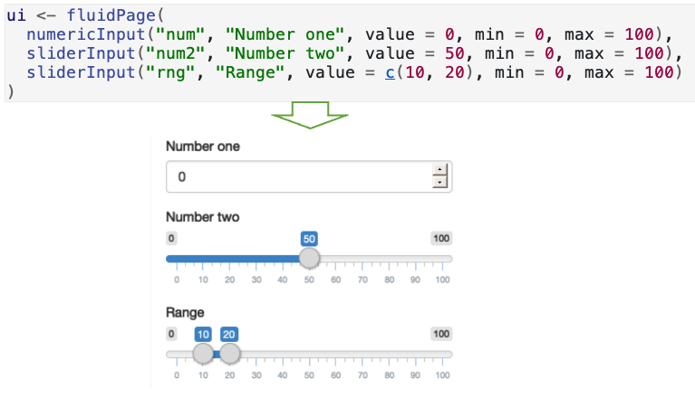
15.8.2 Numeric Inputs
In sliderInput, we can select one or a range of numbers as input. We can also design a dialog box to type a specific number as an input.
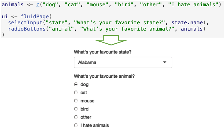
15.8.3 Limited Choices
Whenever a visualization involves a partition based on a discrete variable, selecting a value of a partition variable is useful. There are two different approaches to allow the user to choose from a pre-specified set of options: selectInput() and radioButtons().
15.8.4 File Uploading and Downloading
When working data sets are large or in a special format, uploading and downloading files to Shiny Server becomes necessary. We can design a UI that allows users to upload for analysis and visualization and download the output data. We will cover this topic later.
15.9 Case Study I - Density of Normal Distribution
We revised the previous example and redesigned the layout by including a title, a sidebar, and a main panels. We place three input widgets requesting sample size, the population mean, and standard deviation. The output histogram will be placed in the main panel. The following is the detailed code
library(shiny)

# Define UI for app that draws a histogram ----
ui <- fluidPage(
    # App title ----
    titlePanel("Simulating Standard Normal Distribution"),
    # Sidebar layout with input and output definitions ----
    sidebarLayout(    # siderbarLayout:
         # Sidebar panel for inputs ==> the 1st parameter
         sidebarPanel(
               # Input: Slider for the number of bins ==> 2nd parameter
               sliderInput(inputId = "n",
                           label = "Sample size",
                           min = 1,
                           max = 500,
                           value = 10),
               # slider input: normal population mean
               sliderInput(inputId = "mu",
                           label = "Normal population mean",
                           min = -50,
                           max = 50,
                           value = 0),
               # normal population standard deviation
               sliderInput(inputId = "sigma",
                           label = "Normal population standard deviation",
                           min = 0.1,
                           max = 30,
                           value = 1)),
         # Main panel for displaying outputs ----
         mainPanel(
              # Output: Histogram ----
              plotOutput(outputId = "distPlot")
         )
   ))
# Define server logic required to draw a histogram ----
server <- function(input, output) {
  # Histogram of the simulated normal data ----
  # with requested number of bins
  output$distPlot <- renderPlot({
    # random number generation
    norm.score <- rnorm(input$n, input$mu, input$sigma)
    ##
    hist(norm.score, col = "skyblue", border = "darkred",
         xlab = "Histogram of generated normal data",
         main = "Simulated Normal Distribution")
      })
  }
# Create Shiny app ----
shinyApp(ui = ui, server = server)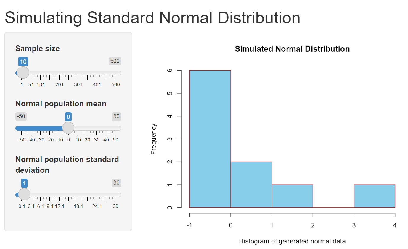
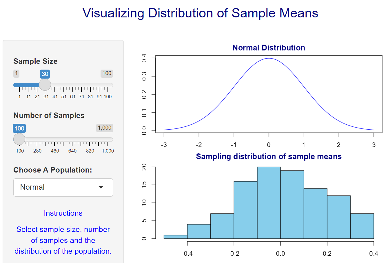
15.10 Case Study 2 - Central Limit Theorem
In this case study, we simulate the sampling distribution of the sample mean (i.e., the central limit theorem)
library(shiny)
# Define UI
ui <- fluidPage(
  # App title ----
  titlePanel(h3("Visualizing Distribution of Sample Means",
             align = "center", style = "color:navy", br(), br())
             ),

  # Sidebar layout with input and output definitions ----
  sidebarLayout(
    # Sidebar panel for inputs ----
    sidebarPanel(
            # Input: Sample size
            p(sliderInput(inputId = "num", "Sample Size",
                        min = 1, max = 100, value = 30),
                        align = "center", style = "color:blue"),
            # Input: number of samples
            sliderInput(inputId = "num2", "Number of Samples",
                        min = 100, max = 1000, value = 100),
            # Input: Selector for populations---
            selectInput(inputId = "dist",
                        label = "Choose A Population:",
                        choices = list("Normal" = 1,
                                       "Uniform" = 2,
                                       "Exponential" = 3,
                                       "Binomial" = 4,
                                       "Poisson" = 5)),
            p("Instructions", align = "center", style = "color:blue"),
            p("Select sample size, number of samples
              and the distribution of the population.",
              align = "center", style = "color:blue")),

    # Main panel for displaying outputs ----
    mainPanel(  # Output: Histogram ----
                 plotOutput(outputId = "distPlot"))
          )
  )

# Define server logic to summarize and view selected dataset ----
server <- function(input, output) {
    ##
    output$distPlot = renderPlot({
           n = input$num      # sample size
        num2 = input$num2     # number of samples
        xbar = NULL           # zero vector with num2 zeroes
        for(i in 1:num2)
           {
             if (input$dist == 1) xbar[i] = mean(rnorm(n))
             if (input$dist == 2) xbar[i] = mean(runif(n))
             if (input$dist == 3) xbar[i] = mean(rexp(n))
             if (input$dist == 4) xbar[i] = mean(rbinom(n,20,0.35))
             if (input$dist == 5) xbar[i] = mean(rpois(n,1.5))
        }
        par(mfrow = c(2,1), mar = c(2, 2, 2, 2))
           if (input$dist == 1) {
               x=seq(-3, 3, length=100)
               plot(x, dnorm(x), type="l", col = "blue",
                    xlab="", ylab="",
                    main="Normal Distribution",
                    col.main = 'navy')
             }
             if (input$dist == 2) {
               x=seq(0, 1, length=100)
               plot(x, dunif(x), type="l", col = "blue",
                    xlab="", ylab="",
                    main="Uniform Distribution",
                    col.main = 'navy')
             }
             if (input$dist == 3) {
               x=seq(0, 6, length=100)
               plot(x, dexp(x), type="l", col = "blue",
                    xlab="", ylab="",
                    main="Exponential Distribution",
                    col.main = 'navy')
             }
             if (input$dist == 4) {
               x = 0:20
               plot(x, dbinom(x, 20, 0.25), type="h", col = "blue",
                    xlab="", ylab="",
                    main="Binomial Distribution",
                    col.main = 'navy')
             }
             if (input$dist == 5) {
               x = 0:8
               plot(x, dpois(x, 1.5), type="h", col = "blue",
                    xlab="", ylab="",
                    main="Poisson Distribution",
                    col.main = 'navy')}
          ###
          hist(xbar, xlab="Random Numbers",
              main = "Sampling distribution of sample means",
              col="skyblue",
              col.main = 'navy')
         })
  }
# Create Shiny app ----
shinyApp(ui, server)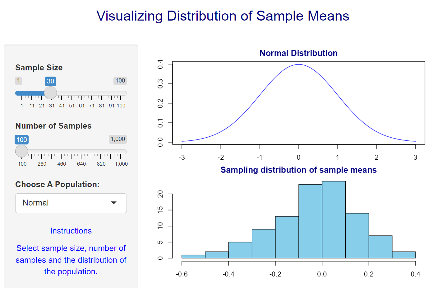
15.11 More Effective Code
library(shiny)
# Define UI
ui <- fluidPage(
  # App title ----
  titlePanel(h3("Visualizing Distribution of Sample Means",
             align = "center", style = "color:navy", br(), br())
             ),

  # Sidebar layout with input and output definitions ----
  sidebarLayout(
    # Sidebar panel for inputs ----
    sidebarPanel(
            # Input: Sample size
            p(sliderInput(inputId = "num", "Sample Size",
                        min = 1, max = 100, value = 30),
                        align = "center", style = "color:blue"),
            # Input: number of samples
            sliderInput(inputId = "num2", "Number of Samples",
                        min = 100, max = 1000, value = 100),
            # Input: Selector for populations---
            selectInput(inputId = "dist",
                        label = "Choose A Population:",
                        choices = list("Normal" = 1,
                                       "Uniform" = 2,
                                       "Exponential" = 3,
                                       "Binomial" = 4,
                                       "Poisson" = 5)),
            p("Instructions", align = "center", style = "color:blue"),
            p("Select sample size, number of samples
              and the distribution of the population.",
              align = "center", style = "color:blue")),

    # Main panel for displaying outputs ----
    mainPanel(  # Output: Histogram ----
                 plotOutput(outputId = "distPlot"))
          )
  )

# Define server logic to summarize and view selected dataset ----
server <- function(input, output) {
    ##
    output$distPlot = renderPlot({
           n = input$num      # sample size
        num2 = input$num2     # number of samples
       par(mfrow = c(2,1), mar = c(2, 2, 2, 2))
       if (input$dist == 1) {
            xbar <- apply(matrix(rnorm(n*num2), ncol=num2),2,mean)
            x=seq(-3, 3, length=100)
            plot(x, dnorm(x), type="l", col = "blue",
            xlab="", ylab="",
            main="Normal Distribution",
            col.main = 'navy')
          }else if (input$dist == 2) {
            xbar <- apply(matrix(runif(n*num2), ncol=num2),2,mean)
            x=seq(0, 1, length=100)
            plot(x, dunif(x), type="l", col = "blue",
                    xlab="", ylab="",
                    main="Uniform Distribution",
                    col.main = 'navy')
          }else if (input$dist == 3) {
            xbar <- apply(matrix(rexp(n*num2), ncol=num2),2,mean)
               x=seq(0, 6, length=100)
               plot(x, dexp(x), type="l", col = "blue",
                    xlab="", ylab="",
                    main="Exponential Distribution",
                    col.main = 'navy')
          }else if (input$dist == 4) {
            xbar <- apply(matrix(rbinom(n*num2,20,0.35), ncol=num2),2,mean)
            x = 0:20
            plot(x, dbinom(x, 20, 0.25), type="h", col = "blue",
                    xlab="", ylab="",
                    main="Binomial Distribution",
                    col.main = 'navy')
          }else if (input$dist == 5) {
            xbar <- apply(matrix(rpois(n*num2,1.5), ncol=num2),2,mean)
            x = 0:8
            plot(x, dpois(x, 1.5), type="h", col = "blue",
                    xlab="", ylab="",
                    main="Poisson Distribution",
                    col.main = 'navy')
          }
          ###
          hist(xbar, xlab="Random Numbers",
              main = "Sampling distribution of sample means",
              col="skyblue",
              col.main = 'navy')
         })
  }
# Create Shiny app ----
shinyApp(ui, server)