Topic 8 Data Processing with Tidyverse
Data visualization is a form of data analysis (also called visual analytics). This means we need to prepare data sets that are appropriate for visualizations. Recall the following work flow of data visualizations mentioned in earlier notes.
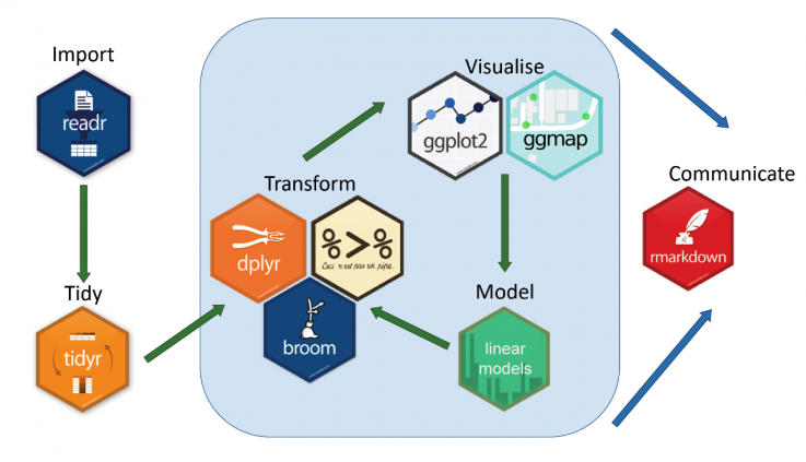
Figure 8.1: Tidyverse workflow.
The major data management tasks are data aggregation and extraction.
Information Aggregation - combining information in different relational data sets to make an integrated single data set for data visualization.
Information Extraction - subsetting a single data set to make small data sets that have specific information for creating a visualization.
The base R package has some powerful and easy-to-use functions to perform these types of data management.
8.1 Data Cleaning and Preparation for Visualization
8.1.1 Data Cleaning
Data cleaning refers to the process of making a data set possibly from different sources of raw data for modeling, visualization, and relevant analysis. The major tasks include:
- Removing unnecessary variables
- Deleting duplicate rows/observations
- Addressing outliers or invalid data
- Dealing with missing values
- Standardizing or categorizing values
- Correcting typographical errors
8.1.2 Data Preparation for Visualization
For a specific data analysis such as modeling or data visualization, we need to create an analytic data set based on clean data sets.
Formatting/Conversion
- Formatting columns appropriately (numbers are treated as numbers, dates as dates)
- Convert values into appropriate units
Filtering/Subsetting
- Filter your data to focus on the specific data that interests you.
- Group data and create aggregate values for groups (Counts, Min, Max, Mean, Median, Mode)
- Extract values from complex columns
Aggregation/Merging
- Combine variables to create new columns
- Merge different relational data sets
8.2 Basic Data Management: Merging Data Sets
There are different packages in R that have various functions capable of doing data management. In this note, we introduce the commonly used functions in base R and tidyverse.
8.2.1 Merge Data Sets
It is very common that the information we are interested in resides in different data sources. In order to merge different data sets, there must be at least one variable “key” that links to different data sets.
There are several different operations in SQL to create different types of the merged data set. The following are the most commonly used ones.
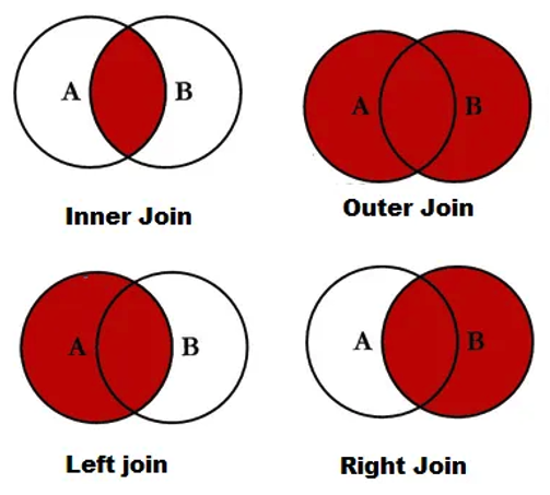
Figure 8.2: Table joins.
The next figure shows the basic operations with tiny tables illustrating the operations.
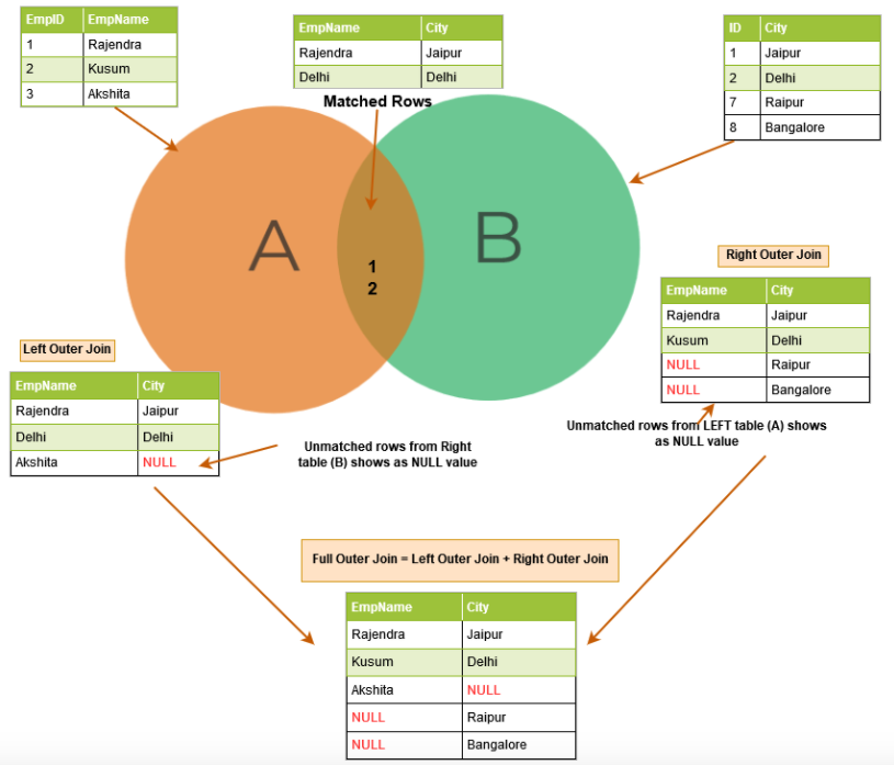
Figure 8.3: An illustrative example of table join.
8.2.2 Merging Data in Base R
The base R function merge() can be used to perform different joins. To illustrate, we use the tiny toy data set in the above figure to show you how to use merge() function.
- Defining Data Frames
employee = data.frame(EmpID = c(1,2,3), EmpName = c("Rajendra", "Kusum", "Akshita"))
city = data.frame(ID = c(1,2,7,8), City =c("Jaipur", "Delhi", "Raipur", "Bangalore"))- Inner Join
##   EmpID  EmpName   City
## 1     1 Rajendra Jaipur
## 2 2 Kusum Delhi- Outer Join
##   EmpID  EmpName      City
## 1     1 Rajendra    Jaipur
## 2     2    Kusum     Delhi
## 3     3  Akshita      <NA>
## 4     7     <NA>    Raipur
## 5 8 <NA> Bangalore- Left Join
##   EmpID  EmpName   City
## 1     1 Rajendra Jaipur
## 2     2    Kusum  Delhi
## 3 3 Akshita <NA>- Right Join
##   EmpID  EmpName      City
## 1     1 Rajendra    Jaipur
## 2     2    Kusum     Delhi
## 3     7     <NA>    Raipur
## 4     8     <NA> Bangalore
8.2.3 Merging Data with Mutating Joins in dplyr
The package dplyr has the following four join functions corresponding to the options in the base R function ’merge()`.
The mutating joins add columns from y to x, matching rows based on the keys:
inner_join(): includes all rows in x and y.left_join(): includes all rows in x.right_join(): includes all rows in y.full_join()(also called outer join): includes all rows in x or y (also called outer join)..
If a row in x matches multiple rows in y, all the rows in y will be returned once for each matching row in x.
To use mutating joins, we first rename key variables so that primary keys have the same name.
employee.new = employee
employee.new$ID = employee$EmpID  # adding the new renamed ID
employee.new = employee.new[, -1]     # drop the old ID variable
employee.new
## EmpName ID
## 1 Rajendra 1
## 2 Kusum 2
## 3 Akshita 3- Inner Join
##    EmpName ID   City
## 1 Rajendra  1 Jaipur
## 2 Kusum 2 Delhi- Left Join
##    EmpName ID   City
## 1 Rajendra  1 Jaipur
## 2    Kusum  2  Delhi
## 3 Akshita 3 <NA>- right Join
##    EmpName ID      City
## 1 Rajendra  1    Jaipur
## 2    Kusum  2     Delhi
## 3     <NA>  7    Raipur
## 4 <NA> 8 Bangalore- Full (Outer) Join
##    EmpName ID      City
## 1 Rajendra  1    Jaipur
## 2    Kusum  2     Delhi
## 3  Akshita  3      <NA>
## 4     <NA>  7    Raipur
## 5     <NA>  8 Bangalore
8.2.4 Use of Pipe Operator %>% with Mutating Joins
The pipe operator, written as %>% takes the output of one function and passes it into another function as an argument. This allows us to link a sequence of analysis steps using functions in dplyr and tidyr in data wrangling.
- Inner Join
##   EmpID  EmpName   City
## 1     1 Rajendra Jaipur
## 2 2 Kusum Delhi- Full (Outer) Join
##   EmpID  EmpName      City
## 1     1 Rajendra    Jaipur
## 2     2    Kusum     Delhi
## 3     3  Akshita      <NA>
## 4     7     <NA>    Raipur
## 5 8 <NA> Bangalore- Left Join
##   EmpID  EmpName   City
## 1     1 Rajendra Jaipur
## 2     2    Kusum  Delhi
## 3 3 Akshita <NA>- Right Join
##   EmpID  EmpName      City
## 1     1 Rajendra    Jaipur
## 2     2    Kusum     Delhi
## 3     7     <NA>    Raipur
## 4     8     <NA> Bangalore
8.3 Basic Data Management: Subsetting Data
Another important data management task is to subset data sets to extract the desired information for analyses and visualization.
Two operations are used to subset a data set: select/drop columns and select rows that meet certain conditions.
The working data set in the section is the well-known iris data set that has 4 numerical variables (attributes of iris flowers) and a categorical variable (species of iris flowers).
8.3.1 Accessors in R [, [[ and $
When subsetting a data set, it is unavoidable to access the value(s) of certain variable(s). Three R accessors are commonly used in R coding.
[subsetting a data set
This R accessor is probably the most commonly used. When we want a subset of an object using [. Remember that when we take a subset of the object you get the same type of thing. Thus, the subset of a vector will be a vector, the subset of a list will be a list and the subset of a data.frame will be a data.frame.
[[extracting one item
The double square brackets are used to extract one element from potentially many. For vectors yield vectors with a single value; data frames give a column vector; for a list, one element:
For example,
## [1] "c"## [1] 1.4 1.4 1.3 1.5 1.4 1.7 1.4 1.5 1.4 1.5 1.5 1.6 1.4 1.1 1.2 1.5 1.3 1.4 1.7 1.5 1.7 1.5 1.0 1.7 1.9 1.6 1.6
## [28] 1.5 1.4 1.6 1.6 1.5 1.5 1.4 1.5 1.2 1.3 1.4 1.3 1.5 1.3 1.3 1.3 1.6 1.9 1.4 1.6 1.4 1.5 1.4 4.7 4.5 4.9 4.0
## [55] 4.6 4.5 4.7 3.3 4.6 3.9 3.5 4.2 4.0 4.7 3.6 4.4 4.5 4.1 4.5 3.9 4.8 4.0 4.9 4.7 4.3 4.4 4.8 5.0 4.5 3.5 3.8
## [82] 3.7 3.9 5.1 4.5 4.5 4.7 4.4 4.1 4.0 4.4 4.6 4.0 3.3 4.2 4.2 4.2 4.3 3.0 4.1 6.0 5.1 5.9 5.6 5.8 6.6 4.5 6.3
## [109] 5.8 6.1 5.1 5.3 5.5 5.0 5.1 5.3 5.5 6.7 6.9 5.0 5.7 4.9 6.7 4.9 5.7 6.0 4.8 4.9 5.6 5.8 6.1 6.4 5.6 5.1 5.6
## [136] 6.1 5.6 5.5 4.8 5.4 5.6 5.1 5.1 5.9 5.7 5.2 5.0 5.2 5.4 5.1The double square bracket looks as if we are asking for something deep within a container. We are not taking a slice but reaching to get at the one thing at the core.
- Interact with
$
The accessor that provides the least unique utility is also probably used the most often used. $ is a special case of [[ in which we access a single item by actual name. The following are equivalent:
##   [1] 1.4 1.4 1.3 1.5 1.4 1.7 1.4 1.5 1.4 1.5 1.5 1.6 1.4 1.1 1.2 1.5 1.3 1.4 1.7 1.5 1.7 1.5 1.0 1.7 1.9 1.6 1.6
##  [28] 1.5 1.4 1.6 1.6 1.5 1.5 1.4 1.5 1.2 1.3 1.4 1.3 1.5 1.3 1.3 1.3 1.6 1.9 1.4 1.6 1.4 1.5 1.4 4.7 4.5 4.9 4.0
##  [55] 4.6 4.5 4.7 3.3 4.6 3.9 3.5 4.2 4.0 4.7 3.6 4.4 4.5 4.1 4.5 3.9 4.8 4.0 4.9 4.7 4.3 4.4 4.8 5.0 4.5 3.5 3.8
##  [82] 3.7 3.9 5.1 4.5 4.5 4.7 4.4 4.1 4.0 4.4 4.6 4.0 3.3 4.2 4.2 4.2 4.3 3.0 4.1 6.0 5.1 5.9 5.6 5.8 6.6 4.5 6.3
## [109] 5.8 6.1 5.1 5.3 5.5 5.0 5.1 5.3 5.5 6.7 6.9 5.0 5.7 4.9 6.7 4.9 5.7 6.0 4.8 4.9 5.6 5.8 6.1 6.4 5.6 5.1 5.6
## [136] 6.1 5.6 5.5 4.8 5.4 5.6 5.1 5.1 5.9 5.7 5.2 5.0 5.2 5.4 5.1## [1] 1.4 1.4 1.3 1.5 1.4 1.7 1.4 1.5 1.4 1.5 1.5 1.6 1.4 1.1 1.2 1.5 1.3 1.4 1.7 1.5 1.7 1.5 1.0 1.7 1.9 1.6 1.6
## [28] 1.5 1.4 1.6 1.6 1.5 1.5 1.4 1.5 1.2 1.3 1.4 1.3 1.5 1.3 1.3 1.3 1.6 1.9 1.4 1.6 1.4 1.5 1.4 4.7 4.5 4.9 4.0
## [55] 4.6 4.5 4.7 3.3 4.6 3.9 3.5 4.2 4.0 4.7 3.6 4.4 4.5 4.1 4.5 3.9 4.8 4.0 4.9 4.7 4.3 4.4 4.8 5.0 4.5 3.5 3.8
## [82] 3.7 3.9 5.1 4.5 4.5 4.7 4.4 4.1 4.0 4.4 4.6 4.0 3.3 4.2 4.2 4.2 4.3 3.0 4.1 6.0 5.1 5.9 5.6 5.8 6.6 4.5 6.3
## [109] 5.8 6.1 5.1 5.3 5.5 5.0 5.1 5.3 5.5 6.7 6.9 5.0 5.7 4.9 6.7 4.9 5.7 6.0 4.8 4.9 5.6 5.8 6.1 6.4 5.6 5.1 5.6
## [136] 6.1 5.6 5.5 4.8 5.4 5.6 5.1 5.1 5.9 5.7 5.2 5.0 5.2 5.4 5.18.3.2 Subsetting Data in Base R
Selecting/Dropping Columns
Subsetting a data set by selecting or dropping a subset of variables (columns) from a data set is straightforward.
For example, we can define a subset of the iris data set by selecting all numerical variables.
##     Sepal.Length Sepal.Width Petal.Length Petal.Width
## 1            5.1         3.5          1.4         0.2
## 2            4.9         3.0          1.4         0.2
## 3            4.7         3.2          1.3         0.2
## 60           5.2         2.7          3.9         1.4
## 61           5.0         2.0          3.5         1.0
## 62           5.9         3.0          4.2         1.5
## 63           6.0         2.2          4.0         1.0
## 110          7.2         3.6          6.1         2.5
## 111          6.5         3.2          5.1         2.0
## 112          6.4         2.7          5.3         1.9
## 113          6.8         3.0          5.5         2.1
We can also create the same data set by dropping variables in the original data set. For example
##     Sepal.Length Sepal.Width Petal.Length Petal.Width
## 1            5.1         3.5          1.4         0.2
## 2            4.9         3.0          1.4         0.2
## 3            4.7         3.2          1.3         0.2
## 60           5.2         2.7          3.9         1.4
## 61           5.0         2.0          3.5         1.0
## 62           5.9         3.0          4.2         1.5
## 63           6.0         2.2          4.0         1.0
## 110          7.2         3.6          6.1         2.5
## 111          6.5         3.2          5.1         2.0
## 112          6.4         2.7          5.3         1.9
## 113          6.8         3.0          5.5         2.1
Selection/Dropping Rows
This is also relatively straightforward. The basic idea is to identify row IDs to select or drop the corresponding rows. The R function which() can this trick!
The following example illustrates the way of using which() to subsetting data.
- Selecting One Species of Iris Flowers
##    Sepal.Length Sepal.Width Petal.Length Petal.Width Species
## 1           5.1         3.5          1.4         0.2  setosa
## 2           4.9         3.0          1.4         0.2  setosa
## 3           4.7         3.2          1.3         0.2  setosa
## 4           4.6         3.1          1.5         0.2  setosa
## 5           5.0         3.6          1.4         0.2  setosa
## 6           5.4         3.9          1.7         0.4  setosa
## 7           4.6         3.4          1.4         0.3  setosa
## 8           5.0         3.4          1.5         0.2  setosa
## 9           4.4         2.9          1.4         0.2  setosa
## 10 4.9 3.1 1.5 0.1 setosa- Selecting Two Species of Iris Flowers
The following three code chunks create the same data set.
Method 1:
not.setosa.id01 = which(iris$Species != "setosa")
not.setosa.flower01 = iris[not.setosa.id01,]
not.setosa.flower01[1:10,]
## Sepal.Length Sepal.Width Petal.Length Petal.Width Species
## 51 7.0 3.2 4.7 1.4 versicolor
## 52 6.4 3.2 4.5 1.5 versicolor
## 53 6.9 3.1 4.9 1.5 versicolor
## 54 5.5 2.3 4.0 1.3 versicolor
## 55 6.5 2.8 4.6 1.5 versicolor
## 56 5.7 2.8 4.5 1.3 versicolor
## 57 6.3 3.3 4.7 1.6 versicolor
## 58 4.9 2.4 3.3 1.0 versicolor
## 59 6.6 2.9 4.6 1.3 versicolor
## 60 5.2 2.7 3.9 1.4 versicolorMethod 2:
not.setosa.id02 = which(iris$Species == "virginica" | iris$Species =="versicolor")
not.setosa.flower02 = iris[not.setosa.id02,]
not.setosa.flower02[1:10,]
## Sepal.Length Sepal.Width Petal.Length Petal.Width Species
## 51 7.0 3.2 4.7 1.4 versicolor
## 52 6.4 3.2 4.5 1.5 versicolor
## 53 6.9 3.1 4.9 1.5 versicolor
## 54 5.5 2.3 4.0 1.3 versicolor
## 55 6.5 2.8 4.6 1.5 versicolor
## 56 5.7 2.8 4.5 1.3 versicolor
## 57 6.3 3.3 4.7 1.6 versicolor
## 58 4.9 2.4 3.3 1.0 versicolor
## 59 6.6 2.9 4.6 1.3 versicolor
## 60 5.2 2.7 3.9 1.4 versicolorMethod 3:
not.setosa.id03 = which(iris$Species %in% c("versicolor", "virginica"))
not.setosa.flower03 = iris[not.setosa.id01,]
not.setosa.flower03[1:10,]
## Sepal.Length Sepal.Width Petal.Length Petal.Width Species
## 51 7.0 3.2 4.7 1.4 versicolor
## 52 6.4 3.2 4.5 1.5 versicolor
## 53 6.9 3.1 4.9 1.5 versicolor
## 54 5.5 2.3 4.0 1.3 versicolor
## 55 6.5 2.8 4.6 1.5 versicolor
## 56 5.7 2.8 4.5 1.3 versicolor
## 57 6.3 3.3 4.7 1.6 versicolor
## 58 4.9 2.4 3.3 1.0 versicolor
## 59 6.6 2.9 4.6 1.3 versicolor
## 60 5.2 2.7 3.9 1.4 versicolor8.3.3 Subsetting Data with dplyr
dplyr provides helper tools for the most common data manipulation tasks. It is built to work directly with data frames and has the ability to work directly with data stored in an external database. We can conduct queries on the database directly and pull back into R only what we need for analysis.
Since selecting/dropping variables is straightforward (particularly when using %>%). Next, we provide a few examples showing how to use filter() to select/drop rows with certain conditions.
- Filtering by one criterion
##    Sepal.Length Sepal.Width Petal.Length Petal.Width Species
## 1           5.1         3.5          1.4         0.2  setosa
## 2           4.9         3.0          1.4         0.2  setosa
## 3           4.7         3.2          1.3         0.2  setosa
## 4           4.6         3.1          1.5         0.2  setosa
## 5           5.0         3.6          1.4         0.2  setosa
## 6           5.4         3.9          1.7         0.4  setosa
## 7           4.6         3.4          1.4         0.3  setosa
## 8           5.0         3.4          1.5         0.2  setosa
## 9           4.4         2.9          1.4         0.2  setosa
## 10          4.9         3.1          1.5         0.1  setosa
## 11          5.4         3.7          1.5         0.2  setosa
## 12          4.8         3.4          1.6         0.2  setosa
## 13          4.8         3.0          1.4         0.1  setosa
## 14          4.3         3.0          1.1         0.1  setosa
## 15          5.8         4.0          1.2         0.2  setosa
## 16          5.7         4.4          1.5         0.4  setosa
## 17          5.4         3.9          1.3         0.4  setosa
## 18          5.1         3.5          1.4         0.3  setosa
## 19          5.7         3.8          1.7         0.3  setosa
## 20          5.1         3.8          1.5         0.3  setosa
## 21          5.4         3.4          1.7         0.2  setosa
## 22          5.1         3.7          1.5         0.4  setosa
## 23          4.6         3.6          1.0         0.2  setosa
## 24          5.1         3.3          1.7         0.5  setosa
## 25          4.8         3.4          1.9         0.2  setosa
## 26          5.0         3.0          1.6         0.2  setosa
## 27          5.0         3.4          1.6         0.4  setosa
## 28          5.2         3.5          1.5         0.2  setosa
## 29          5.2         3.4          1.4         0.2  setosa
## 30          4.7         3.2          1.6         0.2  setosa
## 31          4.8         3.1          1.6         0.2  setosa
## 32          5.4         3.4          1.5         0.4  setosa
## 33          5.2         4.1          1.5         0.1  setosa
## 34          5.5         4.2          1.4         0.2  setosa
## 35          4.9         3.1          1.5         0.2  setosa
## 36          5.0         3.2          1.2         0.2  setosa
## 37          5.5         3.5          1.3         0.2  setosa
## 38          4.9         3.6          1.4         0.1  setosa
## 39          4.4         3.0          1.3         0.2  setosa
## 40          5.1         3.4          1.5         0.2  setosa
## 41          5.0         3.5          1.3         0.3  setosa
## 42          4.5         2.3          1.3         0.3  setosa
## 43          4.4         3.2          1.3         0.2  setosa
## 44          5.0         3.5          1.6         0.6  setosa
## 45          5.1         3.8          1.9         0.4  setosa
## 46          4.8         3.0          1.4         0.3  setosa
## 47          5.1         3.8          1.6         0.2  setosa
## 48          4.6         3.2          1.4         0.2  setosa
## 49          5.3         3.7          1.5         0.2  setosa
## 50 5.0 3.3 1.4 0.2 setosa## Sepal.Length Sepal.Width Petal.Length Petal.Width Species
## 1 7.0 3.2 4.7 1.4 versicolor
## 2 6.4 3.2 4.5 1.5 versicolor
## 3 6.9 3.1 4.9 1.5 versicolor
## 4 6.5 2.8 4.6 1.5 versicolor
## 5 6.3 3.3 4.7 1.6 versicolor
## 6 6.6 2.9 4.6 1.3 versicolor
## 7 6.1 2.9 4.7 1.4 versicolor
## 8 6.7 3.1 4.4 1.4 versicolor
## 9 6.2 2.2 4.5 1.5 versicolor
## 10 6.1 2.8 4.0 1.3 versicolor
## 11 6.3 2.5 4.9 1.5 versicolor
## 12 6.1 2.8 4.7 1.2 versicolor
## 13 6.4 2.9 4.3 1.3 versicolor
## 14 6.6 3.0 4.4 1.4 versicolor
## 15 6.8 2.8 4.8 1.4 versicolor
## 16 6.7 3.0 5.0 1.7 versicolor
## 17 6.7 3.1 4.7 1.5 versicolor
## 18 6.3 2.3 4.4 1.3 versicolor
## 19 6.1 3.0 4.6 1.4 versicolor
## 20 6.2 2.9 4.3 1.3 versicolor
## 21 6.3 3.3 6.0 2.5 virginica
## 22 7.1 3.0 5.9 2.1 virginica
## 23 6.3 2.9 5.6 1.8 virginica
## 24 6.5 3.0 5.8 2.2 virginica
## 25 7.6 3.0 6.6 2.1 virginica
## 26 7.3 2.9 6.3 1.8 virginica
## 27 6.7 2.5 5.8 1.8 virginica
## 28 7.2 3.6 6.1 2.5 virginica
## 29 6.5 3.2 5.1 2.0 virginica
## 30 6.4 2.7 5.3 1.9 virginica
## 31 6.8 3.0 5.5 2.1 virginica
## 32 6.4 3.2 5.3 2.3 virginica
## 33 6.5 3.0 5.5 1.8 virginica
## 34 7.7 3.8 6.7 2.2 virginica
## 35 7.7 2.6 6.9 2.3 virginica
## 36 6.9 3.2 5.7 2.3 virginica
## 37 7.7 2.8 6.7 2.0 virginica
## 38 6.3 2.7 4.9 1.8 virginica
## 39 6.7 3.3 5.7 2.1 virginica
## 40 7.2 3.2 6.0 1.8 virginica
## 41 6.2 2.8 4.8 1.8 virginica
## 42 6.1 3.0 4.9 1.8 virginica
## 43 6.4 2.8 5.6 2.1 virginica
## 44 7.2 3.0 5.8 1.6 virginica
## 45 7.4 2.8 6.1 1.9 virginica
## 46 7.9 3.8 6.4 2.0 virginica
## 47 6.4 2.8 5.6 2.2 virginica
## 48 6.3 2.8 5.1 1.5 virginica
## 49 6.1 2.6 5.6 1.4 virginica
## 50 7.7 3.0 6.1 2.3 virginica
## 51 6.3 3.4 5.6 2.4 virginica
## 52 6.4 3.1 5.5 1.8 virginica
## 53 6.9 3.1 5.4 2.1 virginica
## 54 6.7 3.1 5.6 2.4 virginica
## 55 6.9 3.1 5.1 2.3 virginica
## 56 6.8 3.2 5.9 2.3 virginica
## 57 6.7 3.3 5.7 2.5 virginica
## 58 6.7 3.0 5.2 2.3 virginica
## 59 6.3 2.5 5.0 1.9 virginica
## 60 6.5 3.0 5.2 2.0 virginica
## 61 6.2 3.4 5.4 2.3 virginica- When multiple expressions are used, they are combined using
&(logical AND) or|(logical OR)
##    Sepal.Length Sepal.Width Petal.Length Petal.Width Species
## 1           5.1         3.5          1.4         0.2  setosa
## 2           5.4         3.9          1.7         0.4  setosa
## 3           5.4         3.7          1.5         0.2  setosa
## 4           5.8         4.0          1.2         0.2  setosa
## 5           5.7         4.4          1.5         0.4  setosa
## 6           5.4         3.9          1.3         0.4  setosa
## 7           5.1         3.5          1.4         0.3  setosa
## 8           5.7         3.8          1.7         0.3  setosa
## 9           5.1         3.8          1.5         0.3  setosa
## 10          5.4         3.4          1.7         0.2  setosa
## 11          5.1         3.7          1.5         0.4  setosa
## 12          5.1         3.3          1.7         0.5  setosa
## 13          5.2         3.5          1.5         0.2  setosa
## 14          5.2         3.4          1.4         0.2  setosa
## 15          5.4         3.4          1.5         0.4  setosa
## 16          5.2         4.1          1.5         0.1  setosa
## 17          5.5         4.2          1.4         0.2  setosa
## 18          5.5         3.5          1.3         0.2  setosa
## 19          5.1         3.4          1.5         0.2  setosa
## 20          5.1         3.8          1.9         0.4  setosa
## 21          5.1         3.8          1.6         0.2  setosa
## 22 5.3 3.7 1.5 0.2 setosa## Sepal.Length Sepal.Width Petal.Length Petal.Width Species
## 1 5.1 3.5 1.4 0.2 setosa
## 2 4.9 3.0 1.4 0.2 setosa
## 3 4.7 3.2 1.3 0.2 setosa
## 4 4.6 3.1 1.5 0.2 setosa
## 5 5.0 3.6 1.4 0.2 setosa
## 6 5.4 3.9 1.7 0.4 setosa
## 7 4.6 3.4 1.4 0.3 setosa
## 8 5.0 3.4 1.5 0.2 setosa
## 9 4.4 2.9 1.4 0.2 setosa
## 10 4.9 3.1 1.5 0.1 setosa
## 11 5.4 3.7 1.5 0.2 setosa
## 12 4.8 3.4 1.6 0.2 setosa
## 13 4.8 3.0 1.4 0.1 setosa
## 14 4.3 3.0 1.1 0.1 setosa
## 15 5.8 4.0 1.2 0.2 setosa
## 16 5.7 4.4 1.5 0.4 setosa
## 17 5.4 3.9 1.3 0.4 setosa
## 18 5.1 3.5 1.4 0.3 setosa
## 19 5.7 3.8 1.7 0.3 setosa
## 20 5.1 3.8 1.5 0.3 setosa
## 21 5.4 3.4 1.7 0.2 setosa
## 22 5.1 3.7 1.5 0.4 setosa
## 23 4.6 3.6 1.0 0.2 setosa
## 24 5.1 3.3 1.7 0.5 setosa
## 25 4.8 3.4 1.9 0.2 setosa
## 26 5.0 3.0 1.6 0.2 setosa
## 27 5.0 3.4 1.6 0.4 setosa
## 28 5.2 3.5 1.5 0.2 setosa
## 29 5.2 3.4 1.4 0.2 setosa
## 30 4.7 3.2 1.6 0.2 setosa
## 31 4.8 3.1 1.6 0.2 setosa
## 32 5.4 3.4 1.5 0.4 setosa
## 33 5.2 4.1 1.5 0.1 setosa
## 34 5.5 4.2 1.4 0.2 setosa
## 35 4.9 3.1 1.5 0.2 setosa
## 36 5.0 3.2 1.2 0.2 setosa
## 37 5.5 3.5 1.3 0.2 setosa
## 38 4.9 3.6 1.4 0.1 setosa
## 39 4.4 3.0 1.3 0.2 setosa
## 40 5.1 3.4 1.5 0.2 setosa
## 41 5.0 3.5 1.3 0.3 setosa
## 42 4.5 2.3 1.3 0.3 setosa
## 43 4.4 3.2 1.3 0.2 setosa
## 44 5.0 3.5 1.6 0.6 setosa
## 45 5.1 3.8 1.9 0.4 setosa
## 46 4.8 3.0 1.4 0.3 setosa
## 47 5.1 3.8 1.6 0.2 setosa
## 48 4.6 3.2 1.4 0.2 setosa
## 49 5.3 3.7 1.5 0.2 setosa
## 50 5.0 3.3 1.4 0.2 setosa
## 51 7.1 3.0 5.9 2.1 virginica
## 52 7.6 3.0 6.6 2.1 virginica
## 53 7.3 2.9 6.3 1.8 virginica
## 54 7.2 3.6 6.1 2.5 virginica
## 55 7.7 3.8 6.7 2.2 virginica
## 56 7.7 2.6 6.9 2.3 virginica
## 57 7.7 2.8 6.7 2.0 virginica
## 58 7.2 3.2 6.0 1.8 virginica
## 59 7.2 3.0 5.8 1.6 virginica
## 60 7.4 2.8 6.1 1.9 virginica
## 61 7.9 3.8 6.4 2.0 virginica
## 62 7.7 3.0 6.1 2.3 virginica- To refer to column names that are stored as strings, use the
.datapronoun:
vars <- c("Sepal.Length", "Petal.Length")
cond <- c(6, 5)
subset.iris <- iris %>%
  filter(
    .data[[vars[[1]]]] > cond[[1]],
    .data[[vars[[2]]]] < cond[[2]]
  )
head(subset.iris)
## Sepal.Length Sepal.Width Petal.Length Petal.Width Species
## 1 7.0 3.2 4.7 1.4 versicolor
## 2 6.4 3.2 4.5 1.5 versicolor
## 3 6.9 3.1 4.9 1.5 versicolor
## 4 6.5 2.8 4.6 1.5 versicolor
## 5 6.3 3.3 4.7 1.6 versicolor
## 6 6.6 2.9 4.6 1.3 versicolor8.3.4 Variable Definition and Variable Type Conversion
- Define New Variables
Defining new variables based on the existing variables is straightforward in R using the basic arithmetic and mathematical operations. When using %>%, dplyr() is used to define new variables.
- Variable Type Conversion
Type conversions in R work as you would expect. For example, adding a character string to a numeric vector converts all the elements in the vector to the character.
- Use
is.footo test for data type foo. Returns TRUE or FALSE
is.numeric(), is.character(), is.vector(), is.matrix(), is.data.frame()
- Use
as.footo explicitly convert it.
as.numeric(), as.character(), as.vector(), as.matrix(), as.data.frame)
8.5 Importing Dara
There are different functions in various R libraries to read data to R.
- Base R and Libraries Come with Base R
R loading functions in {utils}: read.table(), read.csv(), read.csv2(), read.delim(), and read.delim2()
- Functions in {tidyverse}
As a part of {tidyverse}, the library {readr} has several functions to read the data in common formats.
read_table(), read_delim(), read_csv(), read_csv2(), read_tsv()
- Read data set generated by other programs such as SAS, SPSS, etc.
Several libraries are useful to load special formats of data to R. Three important libraries are
{xlsx, Hmisc, foreign}.
8.5.1 Exporting Data
We have learned how to use dplyr to extract information from or summarize your raw data, we may want to export these new data sets to share them with other people or for archival.
Similar to the read_csv() function used for reading CSV files into R, there is a write_csv() function that generates CSV files from data frames.
Let’s assume our data set under the name, final_data, is ready, we can save it as a CSV file in our data folder using the following code.
write_csv(final_data, file = "data/final_data.csv")
8.6 Overview of Tidyverse (Optional)
There are several R libraries that have powerful tools for data wrangling and information extraction. Tidyverse is a collection of essential R packages for data science. There 8 packages under the tidyverse umbrella that help us in performing and interacting with the data.
8.6.1 Packages for Data Wrangling and Transformation
dplyr provides helper tools for the most common data manipulation tasks. It is built to work directly with data frames and has the ability to work directly with data stored in an external database. We can conduct queries on the database directly, and pull back into R only what we need for analysis.
tidyr addresses the common problem of wanting to reshape the data with a sophisticated layout for plotting and usage by different R functions.
stringr deals with string variables. It plays a big role in processing raw data into a cleaner and easily understandable format.
forcats is dedicated to dealing with categorical variables or factors. Anyone who has worked with categorical data knows what a nightmare they can be.
8.6.2 Packages for Data Import and Management
tibble is a new modern data frame with nicer behavior around printing, subsetting, and factor handling. It keeps many important features of the original data frame and removes many of the outdated features.
readr package is recently developed to deal with reading in large flat files quickly. The package provides replacements for functions like
read.table()andread.csv().The analogous functions in {readr} areread_table()andread_csv().
8.6.3 Functional Programming with Library {purrr}
- purrr is a new package that fills in the missing pieces in R’s functional programming tools. This is not a coding class. We will not use ‘purrr’ in this class.
8.6.4 Data Visualization and Exploration
ggplot2 is a powerful and flexible R package for producing elegant graphics. The concept behind ggplot2 divides plot into three different fundamental parts: Plot = data + Aesthetics + Geometry.
The principal components of every plot can be defined as follow:
Aesthetics is used to indicate x and y variables. It can also be used to control the color, the size or the shape of points, the height of bars, etc.
Geometry defines the type of graphics (histogram, box plot, line plot, density plot, dot plot, etc.)
This will be one of the primary tools for this class.
8.7 Data Management with dplyr (Optional)
What we can do in the standard SQL can also be done with dyplr. For the convenience of illustration, we use a simple well-known built-in iris data set.
8.7.1 Common dplyr Functions
The following is the list of functions in dplyr.
- select(): sub-setting columns.
To select columns of a data frame, use select(). The first argument to this function is the data frame (iris), and the subsequent arguments are the columns to keep. For example
## 'data.frame':    150 obs. of  3 variables:
##  $ Petal.Length: num  1.4 1.4 1.3 1.5 1.4 1.7 1.4 1.5 1.4 1.5 ...
##  $ Petal.Width : num  0.2 0.2 0.2 0.2 0.2 0.4 0.3 0.2 0.2 0.1 ...
##  $ Species     : Factor w/ 3 levels "setosa","versicolor",..: 1 1 1 1 1 1 1 1 1 1 ...
To select all columns except certain ones, put a “-” in front of the variable to exclude it. For example, we exclude Petal information and only keep Sepal information, we can use the following code
## 'data.frame':    150 obs. of  3 variables:
##  $ Sepal.Length: num  5.1 4.9 4.7 4.6 5 5.4 4.6 5 4.4 4.9 ...
##  $ Sepal.Width : num  3.5 3 3.2 3.1 3.6 3.9 3.4 3.4 2.9 3.1 ...
##  $ Species     : Factor w/ 3 levels "setosa","versicolor",..: 1 1 1 1 1 1 1 1 1 1 ...
This will select all the variables in surveys except for Petal.Length, and Petal.Width.
- filter(): sub-setting rows on conditions.
For example, if we only select one species Versicolor, we can use the following code.
##   Sepal.Length    Sepal.Width     Petal.Length   Petal.Width          Species
##  Min.   :4.900   Min.   :2.000   Min.   :3.00   Min.   :1.000   setosa    : 0
##  1st Qu.:5.600   1st Qu.:2.525   1st Qu.:4.00   1st Qu.:1.200   versicolor:50
##  Median :5.900   Median :2.800   Median :4.35   Median :1.300   virginica : 0
##  Mean   :5.936   Mean   :2.770   Mean   :4.26   Mean   :1.326
##  3rd Qu.:6.300   3rd Qu.:3.000   3rd Qu.:4.60   3rd Qu.:1.500
##  Max.   :7.000   Max.   :3.400   Max.   :5.10   Max.   :1.800
If we subset a data set by selecting a certain number of columns and row with multiple conditions, pipe operator %>% will make subsetting easy. For example, if we only want to study sepal width and length of setosa where petal length is less than 1.5. The following code using %>%
resulting.subset <- iris %>%
             filter(Petal.Length < 1.5, Species =="setosa") %>%
             select(Sepal.Length, Sepal.Width, Species)
summary(resulting.subset)
## Sepal.Length Sepal.Width Species
## Min. :4.300 Min. :2.300 setosa :24
## 1st Qu.:4.600 1st Qu.:3.000 versicolor: 0
## Median :4.900 Median :3.350 virginica : 0
## Mean :4.896 Mean :3.333
## 3rd Qu.:5.100 3rd Qu.:3.525
## Max. :5.800 Max. :4.200Note that, multiple conditional statements are separated by , or &. Using %>%, we don’t need to include the data set as the first argument.
- mutate(): creating new columns by using information from other columns.
Frequently we want to create new columns based on the values in existing columns. For example, we want to define two ratios of the sepal and petal widths and sepal and petal lengths. For this, we’ll use mutate().
expanded.data <- iris %>%
             mutate(length.ratio = Sepal.Length/Petal.Length,
                    width.ratio = Sepal.Width/Petal.Width)
summary(expanded.data)
## Sepal.Length Sepal.Width Petal.Length Petal.Width Species length.ratio width.ratio
## Min. :4.300 Min. :2.000 Min. :1.000 Min. :0.100 setosa :50 Min. :1.050 Min. : 1.130
## 1st Qu.:5.100 1st Qu.:2.800 1st Qu.:1.600 1st Qu.:0.300 versicolor:50 1st Qu.:1.230 1st Qu.: 1.603
## Median :5.800 Median :3.000 Median :4.350 Median :1.300 virginica :50 Median :1.411 Median : 2.148
## Mean :5.843 Mean :3.057 Mean :3.758 Mean :1.199 Mean :2.018 Mean : 6.628
## 3rd Qu.:6.400 3rd Qu.:3.300 3rd Qu.:5.100 3rd Qu.:1.800 3rd Qu.:3.176 3rd Qu.:11.583
## Max. :7.900 Max. :4.400 Max. :6.900 Max. :2.500 Max. :4.833 Max. :41.000- group_by() and summarize(): creating summary statistics on grouped data.
‘group_by()’ is often used together with ‘summarize()’, which collapses each group into a single-row summary of that group. ‘group_by()’ takes as arguments the column names that contain the categorical variables for which you want to calculate the summary statistics.
The following code yields a set of summarized statistics including the mean of sepal width and length as well as the correlation coefficients in each of the three species.
summary.stats <- iris %>%
             group_by(Species) %>%
             summarize(sepal.width.avg = mean(Sepal.Width),
                       sepal.length.avg = mean(Sepal.Length),
                       corr.sepal = cor(Sepal.Length, Sepal.Width))
summary.stats
## # A tibble: 3 × 4
## Species sepal.width.avg sepal.length.avg corr.sepal
## <fct> <dbl> <dbl> <dbl>
## 1 setosa 3.43 5.01 0.743
## 2 versicolor 2.77 5.94 0.526
## 3 virginica 2.97 6.59 0.457All R functions such as min(), max(), , that yield summarized statistics can be used with summarize(). We can also filter out some observations before we compute the summary statistics.
summary.stats.filtering <- iris %>%
             filter(Petal.Length < 5) %>%
             group_by(Species) %>%
             summarize(sepal.width.avg = mean(Sepal.Width),
                       sepal.length.avg = mean(Sepal.Length),
                       corr.sepal = cor(Sepal.Length, Sepal.Width))
summary.stats.filtering
## # A tibble: 3 × 4
## Species sepal.width.avg sepal.length.avg corr.sepal
## <fct> <dbl> <dbl> <dbl>
## 1 setosa 3.43 5.01 0.743
## 2 versicolor 2.77 5.92 0.519
## 3 virginica 2.8 5.85 0.643- arrange(): sorting results.
To sort in descending order, we need to add the desc() function. If we want to sort the results by decreasing the order of mean weight.
summary.stats.sort <- iris %>%
             filter(Petal.Length < 5) %>%
             group_by(Species) %>%
             summarize(sepal.width.avg = mean(Sepal.Width),
                       sepal.length.avg = mean(Sepal.Length),
                       corr.sepal = cor(Sepal.Length, Sepal.Width)) %>%
              arrange(desc(corr.sepal))
summary.stats.sort
## # A tibble: 3 × 4
## Species sepal.width.avg sepal.length.avg corr.sepal
## <fct> <dbl> <dbl> <dbl>
## 1 setosa 3.43 5.01 0.743
## 2 virginica 2.8 5.85 0.643
## 3 versicolor 2.77 5.92 0.519The resulting data set can also be sorted by multiple variables.
- count(): counting discrete values.
When working with data, we often want to know the number of observations found for each factor or combination of factors. For this task, dplyr provides count(). For example, if we wanted to count the number of rows of data for each species after we filter out all records with Petal Length < 5, we would do:
summary.count <- iris %>%
             filter(Petal.Length < 5) %>%
             group_by(Species) %>%
             summarize(count = n(), sort = TRUE)
summary.count
## # A tibble: 3 × 3
## Species count sort
## <fct> <int> <lgl>
## 1 setosa 50 TRUE
## 2 versicolor 48 TRUE
## 3 virginica 6 TRUEIf we wanted to count a combination of factors, say factor A and factor B, we would specify the first and the second factor as the arguments of count(factor A, factor B).
8.7.2 Reshaping Functions in tidyr
The tidyr package complements dplyr perfectly. It boosts the power of dplyr for data manipulation and pre-processing. To illustrate how to use these functions, we consider defining a subset from iris that contains only two variables: Sepal Length and Species.
life.expectancy <-read.csv("https://raw.githubusercontent.com/pengdsci/sta553.html/main/life_expectancy_years.csv")
life.expectancy[1:5, 1:10]
## country X1799 X1800 X1801 X1802 X1803 X1804 X1805 X1806 X1807
## 1 Afghanistan 28.2 28.2 28.2 28.2 28.2 28.2 28.1 28.1 28.1
## 2 Angola 27.0 27.0 27.0 27.0 27.0 27.0 27.0 27.0 27.0
## 3 Albania 35.4 35.4 35.4 35.4 35.4 35.4 35.4 35.4 35.4
## 4 Andorra NA NA NA NA NA NA NA NA NA
## 5 United Arab Emirates 30.7 30.7 30.7 30.7 30.7 30.7 30.7 30.7 30.7sub.iris is called a long table. We can reshape this long table to a wide table using spread() function.
gather(): The function “gathers” multiple columns from the data set and converts them into key-value pairs.
gather()takes four principal arguments:- data set
- the key column variable we wish to create from column names.
- the values column variable we wish to create and fill with values associated with the key.
The names of the columns we use to fill the key variable (or to drop).
Here we exclude country from being gather()ed.
life.expectancy.long <- life.expectancy %>%
  gather(key = "Year",       # the column names of the wide table
         value = "lifeExp",  # the numerical values of the table
         - country,          # drop country variable: its value will not be gathered (stacked)!
         na.rm = TRUE)       # removing records with missing values
##
head(life.expectancy.long)
## country Year lifeExp
## 1 Afghanistan X1799 28.2
## 2 Angola X1799 27.0
## 3 Albania X1799 35.4
## 5 United Arab Emirates X1799 30.7
## 6 Argentina X1799 33.2
## 7 Armenia X1799 34.0We can use substr() to remove X from the variable Year as shown in the following code.
correct.life.exp.data <- life.expectancy.long %>%
                      mutate(year = substr(Year,2,5)) %>%
                      select(-Year)
head(correct.life.exp.data)
## country lifeExp year
## 1 Afghanistan 28.2 1799
## 2 Angola 27.0 1799
## 3 Albania 35.4 1799
## 5 United Arab Emirates 30.7 1799
## 6 Argentina 33.2 1799
## 7 Armenia 34.0 1799For illustrative purposes, we look at a small subset of the iris data set.
##     Sepal.Length Sepal.Width Petal.Length Petal.Width    Species
## 1            5.1         3.5          1.4         0.2     setosa
## 51           7.0         3.2          4.7         1.4 versicolor
## 101          6.3         3.3          6.0         2.5  virginica
We list (select) the columns to be stacked explicitly as arguments of gather() in the following code.
mini.iris.w2l <- mini.iris %>%
          gather(key = "flower.att", value = "measurement",
           Sepal.Length, Sepal.Width, Petal.Length, Petal.Width)
mini.iris.w2l
## Species flower.att measurement
## 1 setosa Sepal.Length 5.1
## 2 versicolor Sepal.Length 7.0
## 3 virginica Sepal.Length 6.3
## 4 setosa Sepal.Width 3.5
## 5 versicolor Sepal.Width 3.2
## 6 virginica Sepal.Width 3.3
## 7 setosa Petal.Length 1.4
## 8 versicolor Petal.Length 4.7
## 9 virginica Petal.Length 6.0
## 10 setosa Petal.Width 0.2
## 11 versicolor Petal.Width 1.4
## 12 virginica Petal.Width 2.5We can also use "-" operator to exclude the column(s) to be gather()ed to make the code cleaner.
mini.iris.w2l0 <- mini.iris %>%
          gather(key = "flower.att", value = "measurement", -Species)
mini.iris.w2l0
## Species flower.att measurement
## 1 setosa Sepal.Length 5.1
## 2 versicolor Sepal.Length 7.0
## 3 virginica Sepal.Length 6.3
## 4 setosa Sepal.Width 3.5
## 5 versicolor Sepal.Width 3.2
## 6 virginica Sepal.Width 3.3
## 7 setosa Petal.Length 1.4
## 8 versicolor Petal.Length 4.7
## 9 virginica Petal.Length 6.0
## 10 setosa Petal.Width 0.2
## 11 versicolor Petal.Width 1.4
## 12 virginica Petal.Width 2.5spread(): takes two columns and “spreads” them into multiple columns. It takes three principal arguments:
- the data
- the key column
(categorical)variable whose values will become new column names. - the value column
(numerical or categorical)variable whose values will fill the new column variables.
Further arguments include filling which, if set, fills in missing values with the value provided.
mini.iris.l2w <- mini.iris.w2l %>%
  spread(key = "flower.att", value = "measurement")
head(mini.iris.l2w)
## Species Petal.Length Petal.Width Sepal.Length Sepal.Width
## 1 setosa 1.4 0.2 5.1 3.5
## 2 versicolor 4.7 1.4 7.0 3.2
## 3 virginica 6.0 2.5 6.3 3.3