Topic 9 Critical Values
As an application of the derivative, we discuss the concept of critical value and its real-world applications in this note.
9.1 Review Topics
We first review the Five Rules of Derivative that will be used frequently throughout the semester.
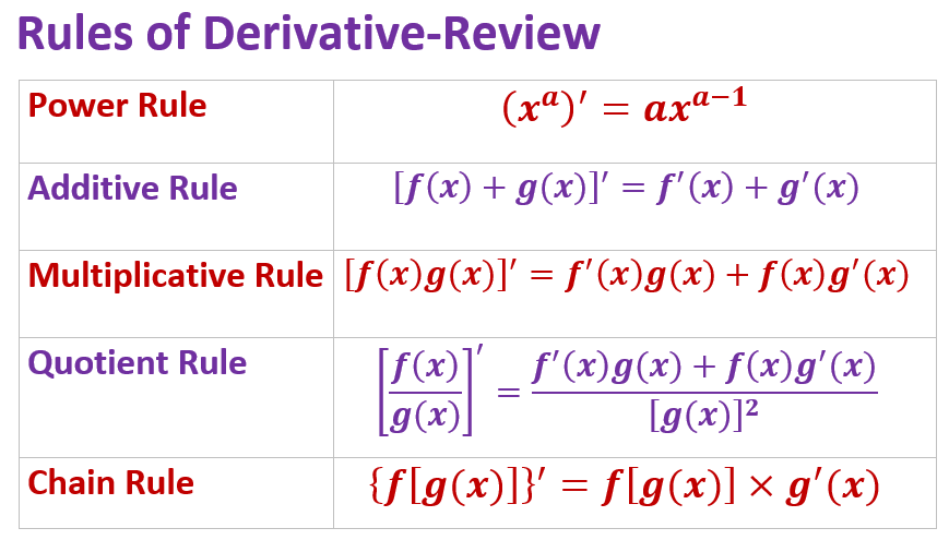
We will apply derivatives to solve real-world optimization problems maximizing profit or revenue and minimizing the cost, etc. This note focuses on the concepts of critical values and using derivation to find critical values.
9.2 Increasing and decreasing functions
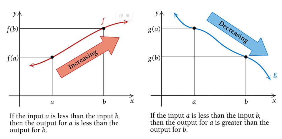
We reviewed monotonic function in the first week. The following figures demonstrate increasing and decreasing functions.
Using the definition of the derivative, we can see that
If \(f(x)\) is increasing over \([a, b]\), then \(f^\prime(x) > 0\) over \([a, b]\);
If \(f(x)\) is decreasing over \([a, b]\), then \(f^\prime(x) < 0\) over \([a, b]\).
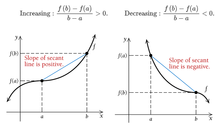
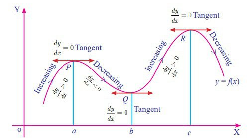
Graphically, we have the following figures explain the above observation
We next formalize the above observation and present the following theorem.
Theorem 1: Let \(f(x)\) be differential over interval \(I = [a,b]\)
If \(f^\prime(x) > 0\) for all x in \(I = [a, b]\), then \(f(x)\) is increasing over \(I=[a, b]\)
If \(f^\prime(x) < 0\) for all x in \(I = [a, b]\), then \(f(x)\) is deceasing over \(I=[a,b]\).
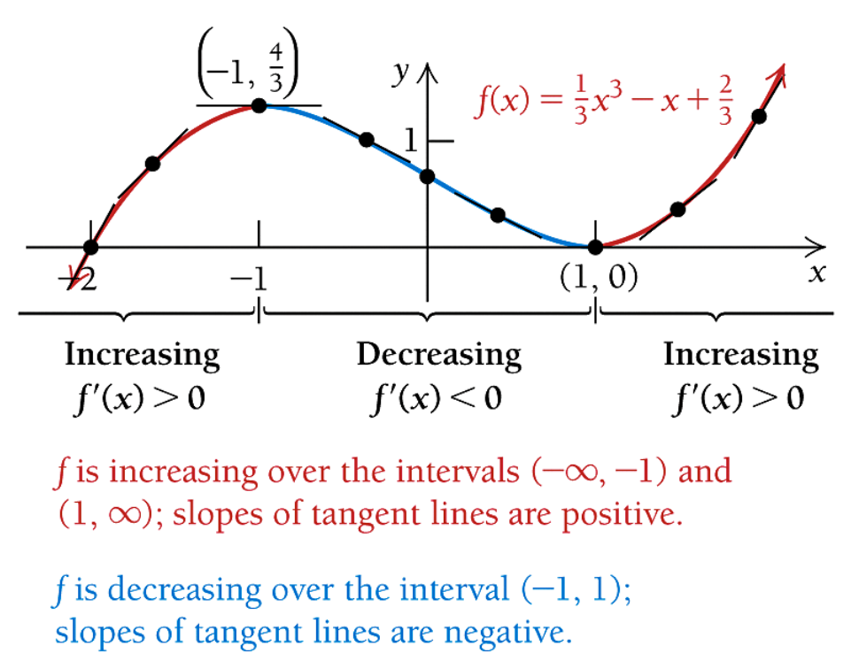
Example 1: Using the above Theorem 1 to find the intervals on which the function \(f(x) = x^3/3 - x + 2/3\).
Solution: The following figure answers the above question.
9.3 Critival Value
In the above curve, two points A and B are special because the monotonicity of the function changed at these points (from increasing to decreasing at A and from decreasing to increasing at B). If the derivative of a function exists over an interval \([a, b]\), if the function changes its monotonicity, its sign of derivative also changes. That means, there exists a value, say \(c\), in \([a, b]\) that satisfies \(f^\prime(c) = 0\).
Definition: A critical value of a function \(f(x)\) is any number \(c\) in the domain of \(f(x)\) for which the tangent line at \((c, f(c))\) is horizontal or for which the derivative does not eixst. That is, \(c\) is a critical value if \(f(c)\) exists and
\[ f^\prime(c) = 0 ~ ~ \text{or}~~ f^\prime(c) ~ \text{does not exist} \] If \(c\) is a critical value of \(f(x)\), then \((c, f(c))\) is called a critical point.
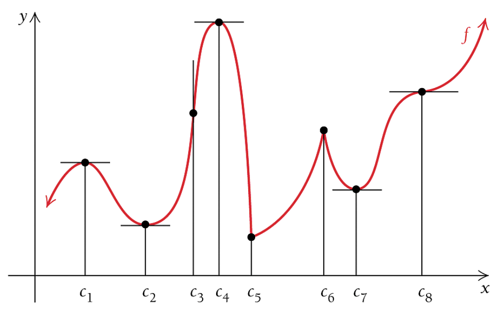
All labeled points on the above figure are critical points since the corresponding derivative is either 0 or does not exist.
\(f^\prime(x) = 0\) for \(x = c_1, c_2, c_4, c_7\) and \(c_8\). That is, the tangent line to the graph is horizontal at these values.
\(f^\prime(x)\) does not exist for \(x = c_3, c_5\) and \(c_6\). The tangent line is vertical at \(c_3\) and there are corners at both \(c_5\) and \(c_6\).
Example 2 Find critical values of the function \(f(x) = x^3/3 - x + 2/3\).
Solution: By the definition, we need to the solution to \(f^\prime(x) = 0\) and those values on which the derivative of \(f(x)\) does not exist.
Note that \(f^\prime(x) = x^2 - 1\). Therefore, equation \(x^2 -1 = 0\) has solutions \(x = \pm 1\). These two critical values are the same as shown in example 1.
9.4 Relative (Local) Maximum and Minimum Values
Graphically, the local maximum and minimum are the second coordinates of the points that are labeled in the following figure.
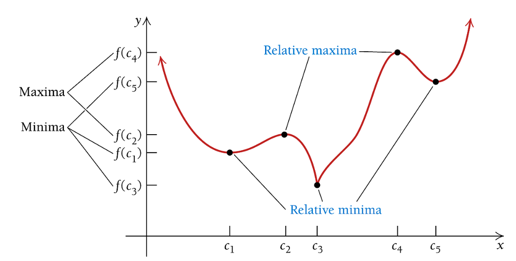
Here, \(f(c_2)\) and \(f(c_4)\) are each an example of a relative, or local, maximum (plural: maxima), and \(f(c_1), f(c_3)\) and \(f(c_5)\) are each an example of a relative, or local, minimum (plural: minima). Collectively, maximum and minimum values are called extrema (singular: extremum). Note that a relative minimum can be greater than a relative maximum; for example, \(f(c_5) > f(c_2)\) in the graph at the bottom of the preceding page.
Note that x-values at which a continuous function has relative extrema are those values for which the derivative is 0 or for which the derivative does not exist—the critical values.
Theorem: If a function \(f(x)\) has a relative extreme value \(f(c)\) on an open interval, then \(c\) is a critical value, and
\[ f^\prime(c) = 0 ~~\text{or}~~f^\prime(c) ~~ \text{does not exist.} \]
The next theorem gives a test for relative extrema: The First-Derivative Test for Relative Extrema
Theorem: For any continuous function \(f(x)\) that has exactly one critical value \(c\) over an open interval \((a, b)\):
\(f(x)\) has a relative minimum at \(c\) if \(f^\prime(x) < 0\) on \((a, c)\) and \(f^\prime(x) > 0\) on \((c, b)\). That is, \(f(x)\) is decreasing to the left of \(c\) and increasing to the right of \(c\).
- \(f(x)\) has a relative maximum at \(c\) if \(f^\prime(x) > 0\) on \((a, c)\) and \(f^\prime(x) < 0\) on \((c, b)\). That is, \(f(x)\) is increasing to the left of \(c\) and decreasing to the right of \(c\).
\(f(x)\) has neither a relative maximum nor a relative minimum at \(c\) if \(f^\prime(x)\) has the same sign on both sides of \(c\).
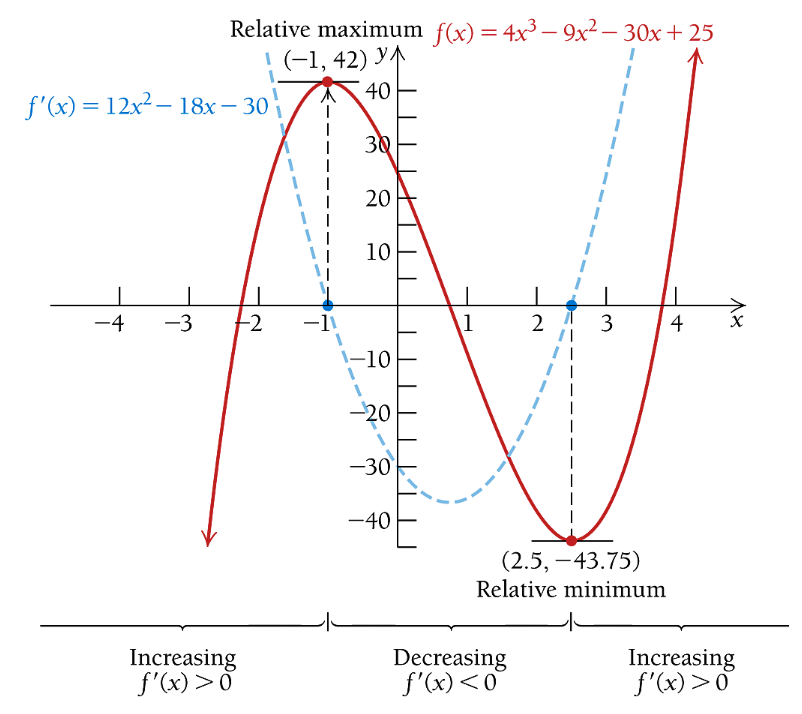
Example 3: Consider the relative maximum and relative minimum of function \(f(x) = 4x^3 - 9x^2 - 30x + 25\).
Solution The derivative \(f^\prime(x) = 12x^2 - 18x -30 = 6(2x^2 - 9x - 5) = 6(ax-5)(x+1)\). Set \(f^\prime(x) = 0\), we have \(6(ax-5)(x+1) = 0\), therefore, \(x = 2.5\) or \(x = -1\).