Topic 16 Applications of Mutivariable Functions

Before discussing the applications of multivariable functions, we review the basics of integral.

Basic Rules and Properties of Integrals.

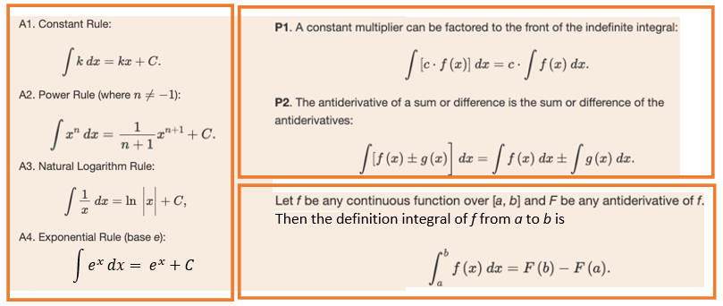
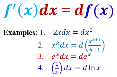
Notations of Differentials

The last example assumes that $x > 0$.

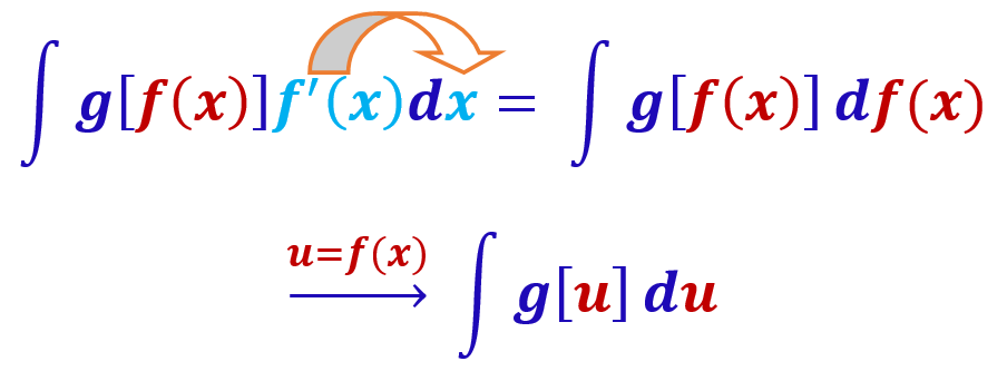
**Integration by Substitution

16.1 More on Partial Derivatives

We first work on two examples of finding the partial derivatives of functions with multiple variables to review the steps and the relevant rules. Then present a pictorial interpretation of partial derivative.

16.1.1 Examples

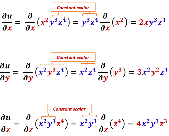
Recall that when taking the derivative of a multivariable function with respect to one variable, all other variables are treated as constant scalars.

Example 1: Find all first order partial derivatives of function $f(x,y,z) = x^2y^3z^4$

Solution: The derivative rule of scalar multiplication will be used repeatedly in the following.

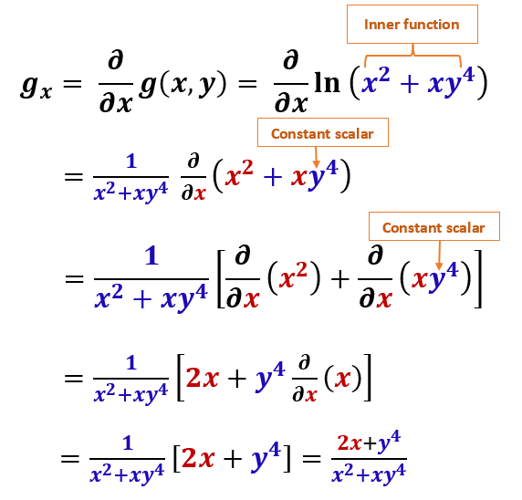
Example 2: Let $g(x,y) = \ln(x^2 + xy^4)$. Find partial derivative $g_x(x,y)$ and $g_y(x,y)$.

Solution: We do the first part. $g_y$ is used for practice.

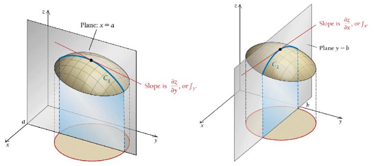
16.1.2 Geometry of Partial Derivatives

The derivative of a single variable function is the slope of the tangent line at $x$. Similarly, a partial derivative also represents the slope of a curve on the surface of the underlying function. The following figure shows the geometry of partial derivatives.

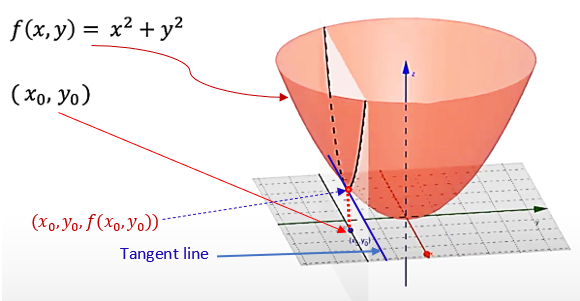
Example 3: Consider the partial derivative $\partial f / \partial x$ of function $f(x,y) = x^2 + y^2$ at $(x_0, y_0)$.

Solution. By definition, the partial derivative of $f(x,y)$ with respect to $x$ is given by \[ \frac{\partial f(x,y)}{\partial x} = \frac{\partial}{\partial x}(x^2 + y^2) = \frac{\partial}{\partial x}(x^2) + \frac{\partial}{\partial x}(y^2)\stackrel{\text{y is a constant}}{=} 2x + 0 = 2x. \]

16.2 Business Applications - Marginal Productivity

One model of production that is frequently in business and economics is the Cobb-Douglass production function \[ p(x,y) = Ax^\alpha y^{1-\alpha}~~\text{for}~~~A>0 ~~~\text{and}~~~ 0<\alpha < 1. \] where $p(x,y)$ is the number of units produced with $x$ units of labor and $y$ units of capital (Capital is the cost of machinery, buildings, tools, and supplies). The partial derivatives

\[ \frac{\partial p(x,y)}{\partial x}~~~\text{and}~~~\frac{\partial p(x,y)}{\partial y} \] are called, respectively, the marginal productivity of labor and the marginal productivity of capital.

Remark: $\alpha$ is a system parameter determined by the production process based on historical production data. It could also be controlled by the management.

Example 4. MyTell Cellular has the following production function for a smartphone: \[ p(x, y)=50x^{2/3} y^{1/3} \] where $p(x,y) is the number of units produced with $x$ units of labor and $y$ units of capital.

1). Find the number of units produced with 125 units of labor and 64 units of capital.

2). Find the marginal productivity.

3). Evaluate the marginal productivity at $x=125$ and $y = 64$.

Solution (1). We simply evaluate the function with the given information about labor and capital.

\[ p(125,64) = 125^{2/3}\times 64^{1/3} = (5^3)^{2/3} \times (4^3)^{1/3} = 5^2\times 4 = 100. \]

(2). We first find the marginal productivity functions of labor and capital respectively in the following.

\[ \frac{\partial p(x,y)}{\partial x} = \frac{\partial}{\partial x}(x^{2/3}y^{1/3}) \stackrel{\text{y is constant}}{=} y^{1/3}\frac{\partial}{\partial x}(x^{2/3}) = y^{1/3}[(2/3)x^{2/3-1}] = \frac{2}{3}x^{-1/3}y^{1/3} \]

\[ \frac{\partial p(x,y)}{\partial y} = \frac{\partial}{\partial y}(x^{2/3}y^{1/3}) \stackrel{\text{x is constant}}{=} x^{2/3}\frac{\partial}{\partial y}(y^{1/3}) = x^{2/3}[(1/3)y^{1/3-1}] = \frac{1}{3}x^{2/3}y^{-2/3} \]

(3). We evaluate the above two partial derivatives respectively in the following

\[ \text{Marginal productivity of labor} = \frac{2}{3}125^{2/3}\times 64^{-1/3} = \frac{2}{3}\times\frac{25}{4} = \frac{25}{6}. \] and

\[ \text{Marginal productivity of capital} = \frac{1}{3}125^{1/3}\times 64^{-2/3} = \frac{1}{3}\times\frac{5}{16} = \frac{5}{48}. \]