Topic 3 Average Rate of Change of A Function
We first review definitions and properties of limits and then introduce the definition of average rate of change of a given function and its technical calculation and geometry.
3.1 Review: Properties of Limits
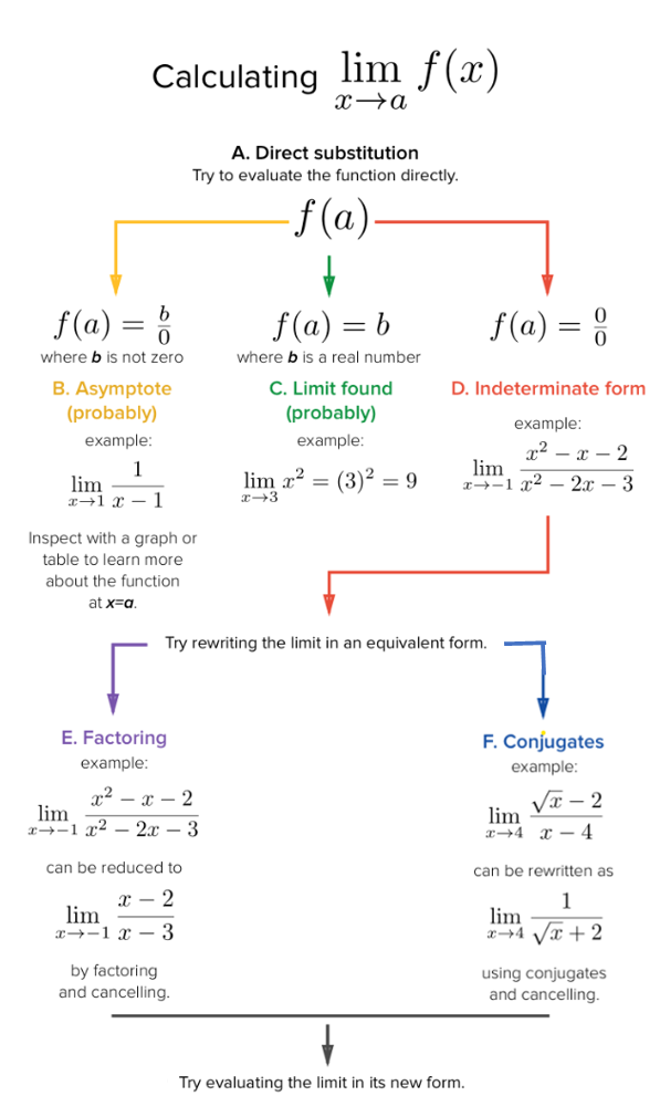
We have described how to find the limit of a function at a given point graphically. Next we introduce how to find limit algebraically. The basic method is substitution. The following chart outlines the workflow in calculating the limit of a given function at a given value of the independent variable.
3.1.1 Sum Rule
This rule states that the limit of the sum of two functions is equal to the sum of their limits: \[ \lim_{x\to a}[f_1(x) + f_2(x) ] = \lim_{x\to a}f_1(x) + \lim_{x\to a}f_2(x). \]
3.1.2 Constant Function Rule
The limit of a constant function is the constant: \[\lim_{x\to a} C = C.\]
3.1.3 Constant Multiple Rule
The limit of constant times a function is equal to the product of the constant and the limit of the function:
\[ \lim_{x\to a}Cf(x) = k\lim_{x\to a}f(x). \]
3.1.4 Product Rule
This rule says that the limit of the product of two functions is the product of their limits (if they exist):
\[ \lim_{x\to a}[f_1(x)f_2(x)] = \lim_{x\to a}f_1(x)\lim_{x\to a}f(x) \]
3.2 Algebraic Calculation of Limits by Examples
Example 1: Compute the value of the following limit \[ \lim_{x\to -2}(3x^2 + 5x -9). \]
Solution:
\[ \lim_{x\to -2}(3x^2 + 5x -9) = 3[\lim_{x\to -2} x]^2 + 5\lim_{x\to -2}x - \lim_{x\to -2}9 = 3\times (-2)^2 + 5(-2) - 9 = -7. \]
Example 2: Evaluate the following limit.
\[ \lim_{x\to 1}\frac{6-3x+10x^2}{-2x^4+7x^3+1}. \] Solution: Using properties of limit, we have
\[ \lim_{x\to 1}\frac{6-3x+10x^2}{-2x^4+7x^3+1}=\frac{\lim_{x\to 1}[6-3x+10x^2]}{\lim_{x\to 1}[-2x^4+7x^3+1]}=\frac{6-3(1)+10(1)^2}{-2(1)^4+7(1)^3+1}=\frac{13}{6}. \]
Example 3 Find the limit
\[ \lim_{x\to 9}\frac{4x^2}{1+\sqrt{x}}. \]
Solution: Using the properties of limits (the sum rule, the power rule, and the quotient rule), we get \[ \lim_{x\to 9}\frac{4x^2}{1+\sqrt{x}}=\frac{\lim_{x\to 9}(4x^2)}{\lim_{x\to 9}(1+\sqrt{x})} = \frac{4\lim_{x\to 9}(x^2)}{(\lim_{x\to 9}1+\lim_{x\to 9}\sqrt{x})} = \frac{4\times 9^2}{(1+\sqrt{9})} = 81. \]
Example 4: Suppose that \(\lim_{x\to 1}f(x) = 2\) and \(\lim_{x \to 1}g(x) = 3\). Calculate the limit
\[ \frac{g(x) - 3f(x)}{f^2(x) + g(x)} \]
Solution: Using the properties of limit, we have \[ \lim_{x\to 1} \frac{g(x) - 3f(x)}{f^2(x) + g(x)} = \frac{\lim_{x\to 1}[g(x) - 3f(x)]}{\lim_{x\to 1}[f^2(x) + g(x)]} = \frac{\lim_{x\to 1}g(x) - 3\lim_{x\to 1}f(x)}{[\lim_{x\to 1}f(x)]^2 + \lim_{x\to 1}g(x)} = -\frac{3}{7}. \]
3.3 Average Rate of Change.
Often times we are not just interested in a function \(f(x)\) itself but also in how \(f(x)\) changes. To be specific, we may be interested in how much the function changed per unit, on average, over an interval.
3.4 Average rate of change of a function over an interval
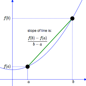
Average rate of change of a function \(f(x)\) over an interval [\(a, b\)] for \(a \ne b\) is defined to be \[ \frac{f(b)-f(a)}{b-a} \] The geometric interpretation of the average rate of change is the slope of the secant line defined based on the interval.
Example: According to Google Maps, it’s about 33 miles from WCU to the Independent Hall in Philadelphia. If Kevin made this trip in 45 minutes, what was his average rate of travel during the trip?
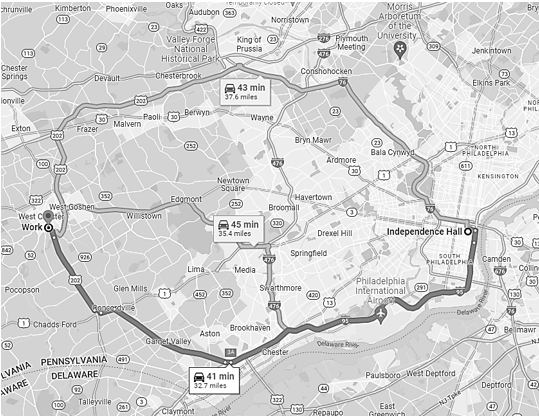
Solution: Let \(t\) be the driving time and \(f(t)\) the driving distance (that is a function of time \(t\)). We set \(t=0\) at the starting point, i.e., \(f(0)=0\). Since it takes 0.75 hours to drive to the destination, this means \(f(0.75) = 33\). Now based on the definition of the rate of change of the distance function \(f(t)\) on interval \([0, 0.75]\), we have \[ V = \frac{f(0.75) - f(0)}{0.75-0} = \frac{33-0}{0.75-0} = \frac{33}{0.75} = 44. \] The rate of change is 44 miles per hour.
Example: In 1998, Linda purchased a house for $144,000. In 2009, the house was worth $245,000. Find the average annual rate of change in dollars per year in the value of the house. Round your answer to the nearest dollar.
Solution: Since house prices (\(P\)) change over time (\(t\)), therefore, house price is a function of time \(P(t)\). The objective is to find the annual rate of change of the house price. It is natural to use the year as the time variable \(t\) and set \(f(1998) = 144000\) and \(f(2009) = 245000\). Then the annual rate of change is \[ \frac{f(2009) - f(1998)}{2009 - 1998} = \frac{245000-144000}{2009-1998} \approx 9182. \]
The annual rate of change is approximately equal to $9182.
3.4.1 Difference quotient
The difference quotient of a (single variable) function is usually the name for the following expression
\[ \frac{f(x+h)-f(x)}{h}. \]
This is a variation of the formula of the rate of change
\[ \frac{f(b)-f(a)}{b -a} \]
where \(a = x\) and \(h = b -a\). We usually assume that \(h\) is close to zero. Without loss of generality, \(h\) is usually assumed to be a small positive number close to zero.
The notation of the difference quotient is easy to use to describe the derivative of a function.
Example: Find the difference quotient of \(f(x) = x^2 + 4x -6\).
Solution: Using the definition of the difference of quotient, we have \[ \frac{f(x+h)-f(x)}{h} = \frac{[(x+h)^2 + 4(x+h) -6]-[x^2+4x-6]}{h}=\frac{2hx+h^2+4h}{h}=2x+h+4. \]
Example: Find the difference quotient of \(f(x) = \sqrt{x}\).
Solution: Using the formula of the difference quotient, we have \[ \frac{\sqrt{x+h}-\sqrt{x}}{h} = \frac{(\sqrt{x+h}-\sqrt{x})(\sqrt{x+h}+\sqrt{x})}{h(\sqrt{x+h}-\sqrt{x})} = \frac{(x+h)-x}{{h(\sqrt{x+h}+\sqrt{x})}} = \frac{1}{\sqrt{x+h}+\sqrt{x}}. \]
Example: Let \(D\) be on the elasticity of demand that is generally defined in the following \[ D = \frac{tC}{P + t} \]
where \(P,t, C\) are respectively price, tax, and constant. We are interested in the effect of the tax change on demand by looking at the difference quotient.
Solution: By the definition of difference quotient, we have \[ \frac{D(t+h) - D(t)}{h} = \frac{\frac{(t+h)C}{P+(t+h)}-\frac{tC}{P+t}}{h} = \frac{(t+h)C}{h(P+t+h)}-\frac{tC}{h(P+t)} \]