Topic 12 Case Study - Logistic regression model with the fraud data

This case study shows how to calculate the local and global performance metrics for logistic predictive models. We have used the confusion matrix in the case study in the previous note. Here we will use the optimal cut-off probability as the decision threshold to define a confusion matrix and then define the performance measure based on this matrix.

We reload the data and create the training and testing data sets. We pretend the optimal cut-off probability is based on what is obtained through the CV. The testing data set will be used to report the local and global performance measures.

fraud.data = read.csv("https://pengdsci.github.io/datasets/FraudIndex/fraudidx.csv")[,-1]
## recode status variable: bad = 1 and good = 0
good.id = which(fraud.data$status == " good") 
bad.id = which(fraud.data$status == "fraud")
##
fraud.data$fraud.status = 0
fraud.data$fraud.status[bad.id] = 1
nn = dim(fraud.data)[1]
train.id = sample(1:nn, round(nn*0.7), replace = FALSE) 
training = fraud.data[train.id,]
testing = fraud.data[-train.id,]

12.1 Local Performance Meaures

Since we have identified the optimal cut-off probability to be 0.57. Next, we will use the testing data set to report the local measures.

test.model = glm(fraud.status ~ index, family = binomial(link = logit), data = training)

## Warning: glm.fit:拟合機率算出来是数值零或一

newdata = data.frame(index= testing$index)
pred.prob.test = predict.glm(test.model, newdata, type = "response")
testing$test.status = as.numeric(pred.prob.test > 0.57)
### components for defining various measures
TN = sum(testing$test.status ==0 & testing$fraud.status==0)
FN = sum(testing$test.status ==0 & testing$fraud.status ==1)
FP = sum(testing$test.status ==1 & testing$fraud.status==0)
TP = sum(testing$test.status ==1 & testing$fraud.status ==1)
###
sensitivity = TP / (TP + FN)
specificity = TN / (TN + FP)
###
precision = TP / (TP + FP)
recall = sensitivity
F1 = 2*precision*recall/(precision + recall)
metric.list = cbind(sensitivity = sensitivity, 
                    specificity = specificity, 
                    precision = precision,
                    recall = recall,
                    F1 = F1)
kable(as.data.frame(metric.list), align='c', caption = "Local performance metrics")

Table 12.1: Local performance metrics

sensitivity	specificity	precision	recall	F1
0.7425021	0.9740736	0.8974625	0.7425021	0.8126612

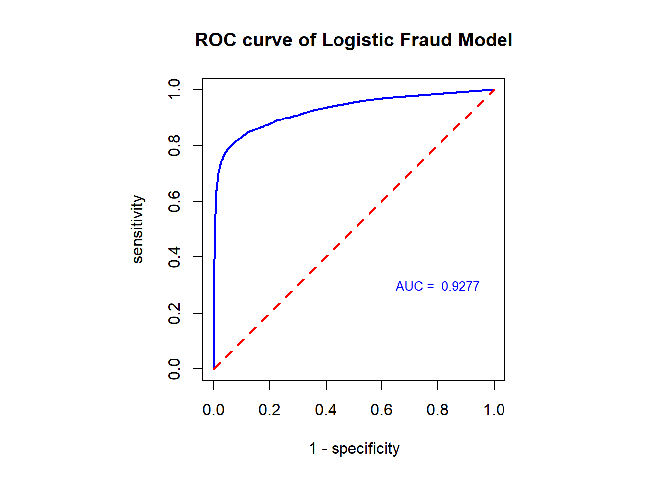
12.2 Global Measure: ROC and AUC

In order to create an ROC curve, we need to select a sequence of decision thresholds and calculate the corresponding sensitivity and specificity.

CAUTION: ROC and AUC are used for model selection, we still use the training data to construct the ROC and calculate the AUC.

cut.off.seq = seq(0, 1, length = 100)
sensitivity.vec = NULL
specificity.vec = NULL
### 
training.model = glm(fraud.status ~ index, family = binomial(link = logit), data = training)

## Warning: glm.fit:拟合機率算出来是数值零或一

newdata = data.frame(index= training$index)
pred.prob.train = predict.glm(training.model, newdata, type = "response")
for (i in 1:100){
  training$train.status = as.numeric(pred.prob.train > cut.off.seq[i])
### components for defining various measures
TN = sum(training$train.status == 0 & training$fraud.status == 0)
FN = sum(training$train.status == 0 & training$fraud.status == 1)
FP = sum(training$train.status == 1 & training$fraud.status == 0)
TP = sum(training$train.status == 1 & training$fraud.status == 1)
###
sensitivity.vec[i] = TP / (TP + FN)
specificity.vec[i] = TN / (TN + FP)
}
one.minus.spec = 1 - specificity.vec
sens.vec = sensitivity.vec
## A better approx of ROC, need library {pROC}
  prediction = pred.prob.train
  category = training$fraud.status == 1
  ROCobj <- roc(category, prediction)

## Setting levels: control = FALSE, case = TRUE

## Setting direction: controls < cases

  AUC = round(auc(ROCobj),4)
##
par(pty = "s")   # make a square figure
plot(one.minus.spec, sens.vec, type = "l", xlim = c(0,1), ylim = c(0,1),
     xlab ="1 - specificity",
     ylab = "sensitivity",
     main = "ROC curve of Logistic Fraud Model",
     lwd = 2,
     col = "blue", )
segments(0,0,1,1, col = "red", lty = 2, lwd = 2)
#AUC = round(sum(sens.vec*(one.minus.spec[-101]-one.minus.spec[-1])),4)
text(0.8, 0.3, paste("AUC = ", AUC), col = "blue", cex = 0.8)