Topic 8 Basics of Bootstrap Method
The bootstrap method is a data-based simulation method for statistical inference. The method assumes that
The sample is a random sample representing the population;
The sample size is large enough such that the empirical distribution can be close to the true distribution.
8.1 Basic Idea of Bootstrap Method.
The objective is to estimate a population parameter such as mean, variance, correlation coefficient, regression coefficients, etc. from a random sample without assuming any probability distribution of the underlying distribution of the population.
For convenience, we assume that the population of interest has a cumulative distribution function \(F(x: \theta)\), where \(\theta\) is a vector of the population. For example, You can think about the following distributions
Normal distribution: \(N(\mu, \sigma^2)\), the distribution function is given by
\[f(x:\theta) = \frac{1}{\sqrt{2\pi}\sigma}\exp\left(-\frac{(x-\mu)^2}{2\sigma^2}\right)\] where \(\theta = (\mu, \sigma)\). Since the normal distribution is so fundamental in statistics, we use the special notation for the cumulative distribution \(\phi_{\mu, \sigma^2}(x)\) or simply \(\phi(x)\). The corresponding probability function
Binomial distribution: \(Binom(n, p)\), the probability distribution is given by
\[ P(x) = \frac{n!}{x!(n-x)!}p^x(1-p)^{n-x}, x = 0, 1, 2, \cdots, n-1, n.\] where \(\theta = p\). Caution: \(n\) is NOT a parameter!
We have already learned how to make inferences about population means and variances under various assumptions in elementary statistics. In this note, we introduce a new approach to making inferences only based on a given random sample taken from the underlying population.
As an example, we focus on the population mean. For other parameters, we can follow the same idea to make bootstrap inferences.
8.1.1 Random Sample from Population
We have introduced various study designs and sampling plans to obtain random samples from a given population with the distribution function \(F(x:\theta)\). Let \(\mu\) be the population mean.
- Random Sample. Let
\[\{x_1, x_2, \cdots, x_n\} \to F(x:\theta)\] be a random sample from population \(F(x:\theta)\).
- Sample Mean. The point estimate is given by
\[\hat{\mu} = \frac{\sum_{i=1}^n x_i}{n}\]
Sampling Distribution of \(\hat{\mu}\). In order to construct the confidence interval of \(\mu\) or make hypothesis testing about \(\mu\), we need to know the sampling distribution of \(\hat{\mu}\). From elementary statistics, we have the following results.
\(\hat{\mu}\) is normally distributed if (1). \(n\) is large; or (2). the population is normal and population variance is known.
the standardized \(\hat{\mu}\) follows a t-distribution if the population is normal and population variance is unknown.
\(\hat{\mu}\) is unknown of the population is not normal and the sample size is not large enough.
In the last case of the previous bullet point, we don’t have the theory to derive the sampling distribution based on a single sample. However, if the sampling is not too expensive and time-consuming, we take following the sample study design and sampling plan to repeatedly take a large number, 1000, samples of the same size from the population. We calculate the mean of each of the 1000 samples and obtain 1000 sample means \(\{\hat{\mu}_1, \hat{\mu}_2, \cdots, \hat{\mu}_{1000}\}\). Then the empirical distribution of \(\hat{\mu}\).
The following figure depicts how to approximate the sampling distribution of the point estimator of the population parameter.
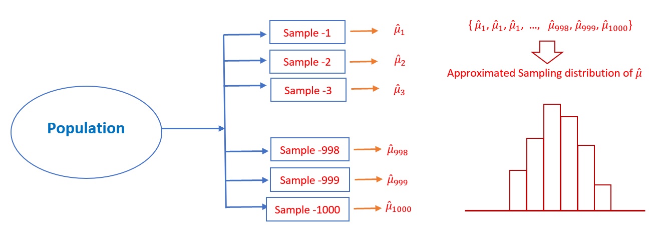
Figure 8.1: Figure 1. Steps for estimating the sampling distribution of a point estimator of the population parameter
Example 1: [Simulated data] Assume that the particular numeric characteristics of the WCU student population are the heights of all students.
We don’t know the distribution of the heights.
We also don’t know whether a specific sample size is large enough to use the central limit theorem. This means we don’t know whether it is appropriate to use the central limit theorem to characterize the sampling distribution of the mean height.
Due to the above constraints, we cannot find the sampling distribution of the sample mean using only the knowledge of elementary statistics. However, if sampling is not expensive, we take repeated samples with the same sample size. The resulting sample means can be used to approximate the sampling distribution of the sample mean.
Next, we use R and the simulated data set https://pengdsci.github.io/STA551/w05/w05-wcuheights.txt to implement the above idea. I will use simple code with comments to explain the task of each line of code so you can easily understand the coding logic.
# read the delimited data from URL
wcu.height = read.table("https://pengdsci.github.io/STA551/w05/w05-wcuheights.txt", header = TRUE)
sample.mean.vec = NULL      # define an empty vector to hold sample means of repeated samples.
for(i in 1:1000){           # starting for-loop to take repeated random samples with n = 81
  ith.sample = sample( wcu.height$Height,       # population of all WCU students heights
                       81,                      # sample size = 81 values in the sample
                       replace = FALSE          # sample without replacement
                 )                              # this is the i-th random sample
   sample.mean.vec[i] = mean(ith.sample)        # calculate the mean of i-th sample and save it in
                                                # the empty vector: sample.mean.vec
  }
Next, we make a histogram of the sample means saved in sample.mean.vec.
hist(sample.mean.vec,                                               # data used for histogram
     breaks = 14,                                                   # specify the number of vertical bars
     xlab = "sample means of repeated samples",                     # change the label of x-axis
     main="Approximated Sampling Distribution of the Sample Mean")   # add a title to the histogram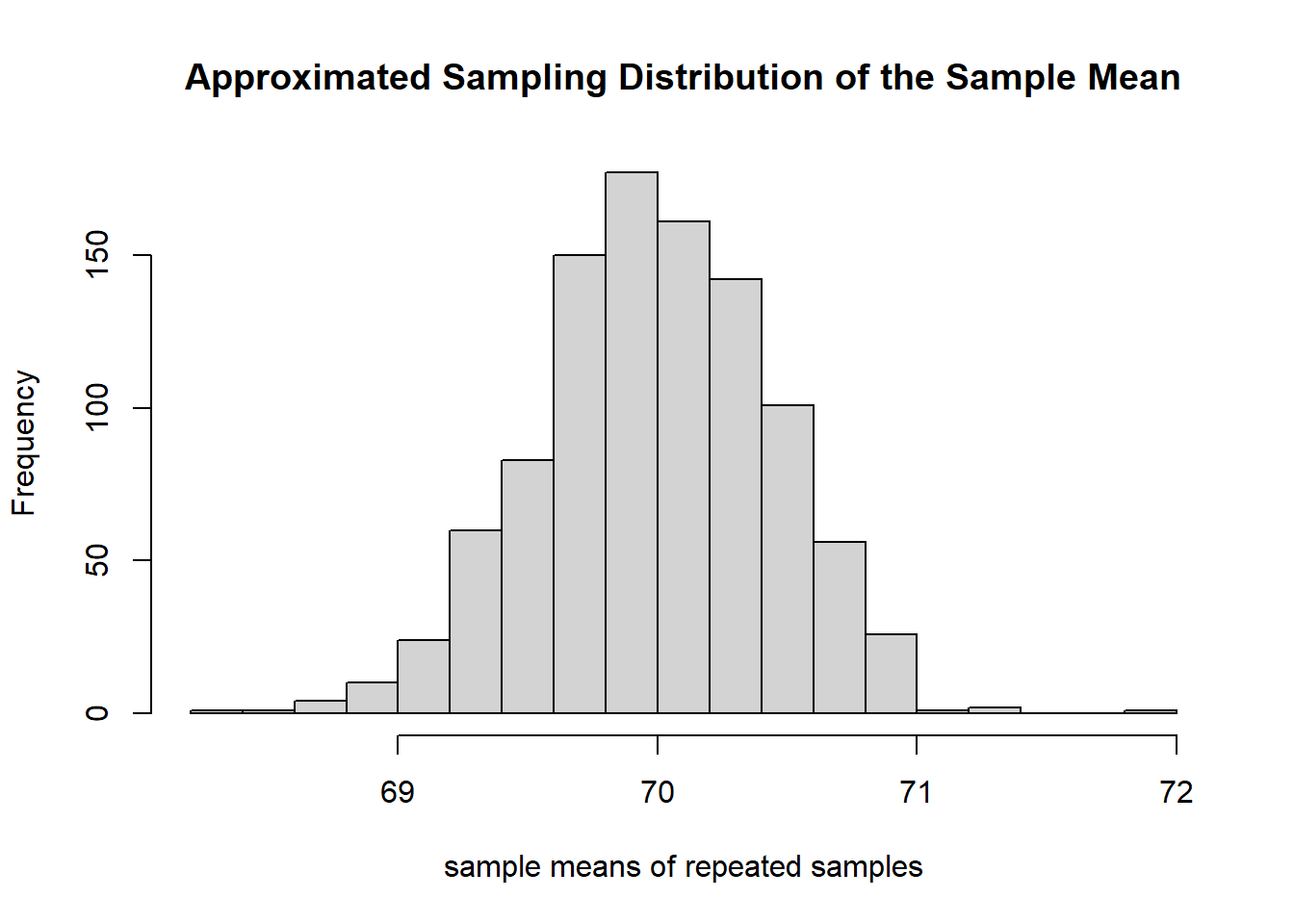
Figure 8.2: Figure 2. Approximated sampling distribution of sample mean used the repeated samples.
8.1.2 Bootstrap Sampling and Bootstrap Sampling Distribution
Recall the situation in Example 1 in which we were not able to use the normality assumption of the population and the central limit theorem (CLT) but were allowed to take repeated samples from the population. In practice, taking samples from the population can be very expensive. Is there any way to estimate the sampling distribution of the sample mean? The answer is YES under the assumption the sample yields a valid estimation of the original population distribution.
Bootstrap Sampling With the assumption that the sample yields a good approximation of the population distribution, we can take bootstrap samples from the actual sample. Let \[\{x_1, x_2, \cdots, x_n\} \to F(x:\theta)\] be the actual random sample taken from the population. A bootstrap sample is obtained by taking a sample with replacement from the original data set (not the population!) with the same size as the original sample. Because with replacement was used, some values in the bootstrap sample appear once, some twice, and so on, and some do not appear at all.
Notation of Bootstrap Sample. We use \(\{x_1^{(i*)}, x_2^{(i*)}, \cdots, x_n^{(i*)}\}\) to denote the \(i^{th}\) bootstrap sample. Then the corresponding mean is called bootstrap sample mean and denoted by \(\hat{\mu}_i^*\), for \(i = 1, 2, ..., n\).
Bootstrap sampling distribution of the sample mean can be estimated by taking a large number, say B, of bootstrap samples. The resulting B bootstrap sample means are used to estimate the sampling distribution. Note that, in practice, B is bigger than 1000.
The above Bootstrap sampling process is illustrated in the following figure.
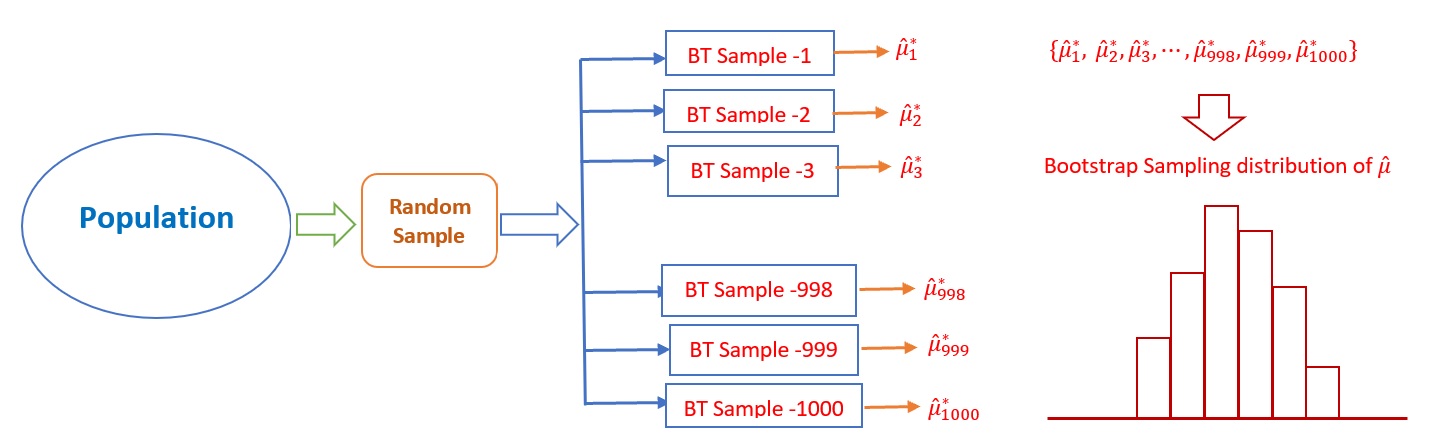
Figure 8.3: Steps for the Bootstrap sampling distribution of a point estimator of the population parameter
- Example 2: [continue to use WCU Heights]. We use the Bootstrap method to estimate the sampling distribution of the sample mean.
### Read the delimited data from the URL
wcu.height = read.table("https://pengdsci.github.io/STA551/w05/w05-wcuheights.txt", header = TRUE)
# taking the original random sample from the population
original.sample = sample( wcu.height$Height,    # population of all WCU students heights
                       81,                      # sample size = 81 values in the sample
                       replace = FALSE          # sample without replacement
                 )
### Bootstrap sampling begins
bt.sample.mean.vec = NULL      # define an empty vector to hold sample means of repeated samples.
for(i in 1:1000){              # starting for-loop to take bootstrap samples with n = 81
  ith.bt.sample = sample( original.sample,    # Original sample with 81 WCU students' heights
                       81,                    # sample size = 81 MUST be equal to the sample size!!
                       replace = TRUE         # MUST use WITH REPLACEMENT!!
                 )                            # This is the i-th Bootstrap sample
  bt.sample.mean.vec[i] = mean(ith.bt.sample) # calculate the mean of i-th bootstrap sample and
                                              # save it in the empty vector: sample.bt.mean.vec
  }
The following histogram shows the bootstrap sampling distribution of the sample with size \(n=81\).
hist(bt.sample.mean.vec,                                         # data used for histogram
     breaks = 14,                                                # specify the number of vertical bars
     xlab = "Bootstrap sample means",                            # change the label of x-axis
     main="Bootstrap Sampling Distribution of the Sample Mean")   # add a title to the histogram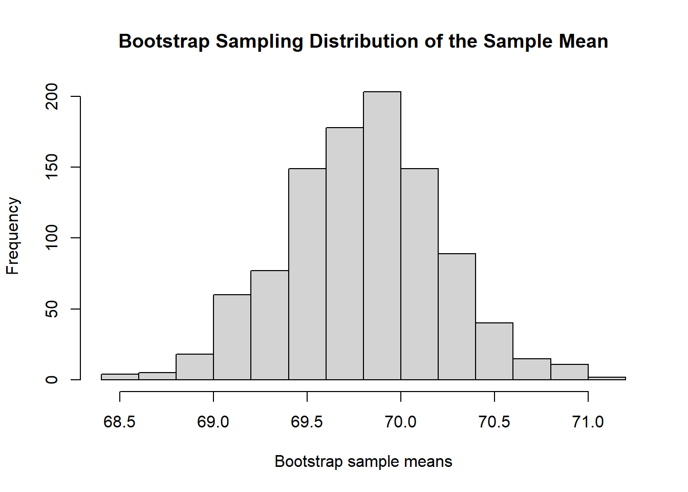
Figure 8.4: Figure 4. Bootstrap sampling distribution of sample means
8.1.3 Relationship between Two Estimated Sampling Distributions
We can see that the two sampling distributions are slightly different. If we are allowed to take repeated samples from the population, we should always use the repeated sample approach since it yields a better estimate of the true sampling distribution.
The bootstrap estimate of the sampling distribution is used when no theoretical confidence intervals are unavailable and the repeated sample is not possible. This does not mean that the bootstrap methods do not have limitations. In fact, the implicit assumption of the bootstrap method is that the original sample has enough information to estimate the true population distribution.
8.2 Bootstrap Confidence Intervals
First of all, all bootstrap confidence intervals are constructed based on the bootstrap sampling distribution of the underlying point estimator of the parameter of interest.
There are at least five different bootstrap confidence intervals. You can find these definitions from Chapter 4 of Roff’s eBook https://ebookcentral.proquest.com/lib/wcupa/reader.action?docID=261114&ppg=7 (need WCU login credential to access the book). We only focus on the percentile method in which we simply define the confidence limit(s) by using the corresponding percentile(s) of the bootstrap estimates of the parameter of interest. R has a built-in function, quantile(), to find percentiles.
- Example 3: We construct a 95% two-sided bootstrap percentile confidence interval of the mean height of WCU students. This is equivalent to finding the 2.5% and 97.5% percentiles. We use the following one-line code.
##     2.5%    97.5%
## 68.99938 70.64198Various bootstrap methods were implemented in the R library {boot}. UCLA Statistical Consulting https://stats.idre.ucla.edu/r/faq/how-can-i-generate-bootstrap-statistics-in-r/ has a nice tutorial on bootstrap confidence intervals. You can use the built-in function boot.ci() to find all 5 bootstrap confidence intervals after you create the boot object. I will leave it to you if you want to explore more about the library.
8.3 Bootstrap Confidence Interval of Correlation Coefficient
As a case study, we will illustrate one bootstrap method to sample a random sample with multiple variables and use the bootstrap samples to calculate the corresponding bootstrap correlation coefficient. The bootstrap percentile confidence interval of the correlation coefficient.
8.3.1 Bootstrapping Data Set
There are different ways to take bootstrap samples. The key point is that we cannot sample individual variables in the data frame separately to avoid mismatching! The method we introduce here is also called bootstrap sampling cases. Here are the basic steps:
We define the vector of row \(ID\). That is, \(ID = \{1, 2, 3, ..., n\}\).
Take a bootstrap sample from \(ID\) (i.e., sampling with replacement) with same size = n, denoted by \(ID^*\). As commented earlier, there will be replicates in \(ID^*\) and some values in \(ID\) are not in \(ID^*\).
Use \(ID^*\) to select the corresponding rows to form a bootstrap sample and then perform bootstrap analysis.
Here is an example of taking the bootstrap sample from the original sample with multiple variables. The data set we use here is well-known and is available at https://pengdsci.github.io/STA551/w05/w05-iris.txt
# read data into R from URL:
iris = read.table("https://pengdsci.github.io/STA551/w05/w05-iris.txt", header = TRUE)
n = dim(iris)[1]        # returns the dimension of the data frame, 1st component is the number of rows
bt.ID = sample(1:n, replace = TRUE)   # bootstrap IDs, MUST use replacement method!
sort(bt.ID)                 # check the content of bt.ID. I sort the bt.ID to see the replicate easily
## [1] 2 2 3 3 3 4 5 7 8 8 8 10 10 11 13 13 15 17 17 17 17 18 19 19 19 21 22 22
## [29] 23 23 24 25 25 25 25 26 27 27 28 31 32 34 34 34 35 35 37 38 40 40 43 44 45 47 47 47
## [57] 48 48 50 51 52 53 54 54 55 57 60 61 61 62 66 67 67 67 67 68 68 71 72 74 76 77 78 79
## [85] 79 81 81 82 86 87 87 87 88 88 88 88 88 90 91 92 92 92 94 96 99 99 100 101 102 103 105 106
## [113] 106 111 111 111 114 118 119 120 120 121 121 122 124 125 127 127 128 130 130 130 131 132 136 138 138 138 139 140
## [141] 140 140 142 143 143 147 147 147 148 150Next, we use the above bt.ID to take the bootstrap sample from the original data set iris.
8.3.2 Confidence Interval of Coefficient Correlation
In this section, we construct a 95% bootstrap percentile confidence interval for the coefficient correlation between the SepalLength and SepalWidth given in iris. Note that R built-in function cor(x,y) can be used to calculate the bootstrap correlation coefficient directly. The R code for constructing the bootstrap confidence interval for the coefficient correlation is given below.
iris = read.table("https://pengdsci.github.io/STA551/w05/w05-iris.txt", header = TRUE)
n = dim(iris)[1]        # returns the dimension of the data frame, 1st component is the number of rows
##
bt.cor.vec = NULL    # empty vector bootstrap correlation coefficients
for (i in 1:5000){   # this time I take 5000 bootstrap samples for this example.
  bt.ID.i = sample(1:n, replace = TRUE)  # bootstrap IDs, MUST use replacement method!
  bt.iris.i = iris[bt.ID.i, ]            # i-th bootstrap ID
  bt.cor.vec[i] = cor(bt.iris.i$SepalLength, bt.iris.i$SepalWidth)   # i-th bootstrap correlation coefficient
}
bt.CI = quantile(bt.cor.vec, c(0.025, 0.975) )
bt.CI
## 2.5% 97.5%
## -0.25324764 0.03440942Interpretation: We are 95% confident that there is no statistically significant correlation between sepal length and sepal width based on the given sample. This may be because the data set contains three different types of iris.
Next, we make two plots to visualize the relationship between the two variables.
par(mfrow=c(1,2))   # Layout a plot sheet: 1 row and 2 columns
## histogram
hist(bt.cor.vec, breaks = 14,
       main="Bootstrap Sampling \n  Distribution of Correlation",
      xlab = "Bootstrap Correlation Coefficient")
## scatter plot
plot(iris$SepalLength, iris$SepalWidth,
     main = "Sepal Length vs Width",
     xlab = "Sepal Length",
     ylab = "Sepal Width")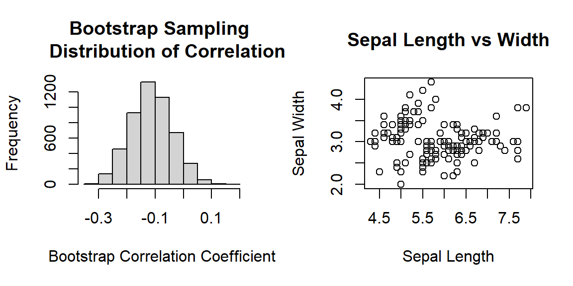
Figure 8.5: Left panel: histogram of the bootstrap coefficient of correlation. Right panel: the scatter plot of the sepal length and width.