Topic 15 Time Series Decomposition
Time series decomposition is a process of splitting a time series into basic components: trend, seasonality random error. The method originated a century ago and new developments in the past few decades.
Seasonal: Patterns that repeat for a fixed period. For example, a website might receive more visits during weekends; this would produce data with seasonality of 7 days.
Trend: The underlying trend of the metrics. A website increasing in popularity should show a general trend that goes up.
Random Error: Also call “noise”, “residual” or “remainder”. These are the residuals of the original time series after the seasonal and trend series are removed.
The objective of time series decomposition is to model the trend and seasonality and estimate the overall time series as a combination of them. A seasonally adjusted value removes the seasonal effect from a value so that trends can be seen more clearly.
The following two working data sets were widely used in different textbooks. We will use them to illustrate some of the concepts.
Australian Beer Production Data
The following data gives quarterly beer production figures in Australia from 1956 through the 2nd quarter of 2010. The beer production figure is in megalitres.
ausbeer0=c(284, 213, 227, 308, 262, 228, 236, 320, 272, 233, 237, 313, 261, 227, 250, 314,
          286, 227, 260, 311, 295, 233, 257, 339, 279, 250, 270, 346, 294, 255, 278, 363,
          313, 273, 300, 370, 331, 288, 306, 386, 335, 288, 308, 402, 353, 316, 325, 405,
          393, 319, 327, 442, 383, 332, 361, 446, 387, 357, 374, 466, 410, 370, 379, 487,
          419, 378, 393, 506, 458, 387, 427, 565, 465, 445, 450, 556, 500, 452, 435, 554,
          510, 433, 453, 548, 486, 453, 457, 566, 515, 464, 431, 588, 503, 443, 448, 555,
          513, 427, 473, 526, 548, 440, 469, 575, 493, 433, 480, 576, 475, 405, 435, 535,
          453, 430, 417, 552, 464, 417, 423, 554, 459, 428, 429, 534, 481, 416, 440, 538,
          474, 440, 447, 598, 467, 439, 446, 567, 485, 441, 429, 599, 464, 424, 436, 574,
          443, 410, 420, 532, 433, 421, 410, 512, 449, 381, 423, 531, 426, 408, 416, 520,
          409, 398, 398, 507, 432, 398, 406, 526, 428, 397, 403, 517, 435, 383, 424, 521,
          421, 402, 414, 500, 451, 380, 416, 492, 428, 408, 406, 506, 435, 380, 421, 490,
          435, 390, 412, 454, 416, 403, 408, 482, 438, 386, 405, 491, 427, 383, 394, 473,
420, 390, 410)- Airline Passengers Data
This data set records monthly totals of international airline passengers (1949-1960).
AirPassengers0=c(112, 118, 132, 129, 121, 135, 148, 148, 136, 119, 104, 118, 115, 126, 141,
                135, 125, 149, 170, 170, 158, 133, 114, 140, 145, 150, 178, 163, 172, 178,
                199, 199, 184, 162, 146, 166, 171, 180, 193, 181, 183, 218, 230, 242, 209,
                191, 172, 194, 196, 196, 236, 235, 229, 243, 264, 272, 237, 211, 180, 201,
                204, 188, 235, 227, 234, 264, 302, 293, 259, 229, 203, 229, 242, 233, 267,
                269, 270, 315, 364, 347, 312, 274, 237, 278, 284, 277, 317, 313, 318, 374,
                413, 405, 355, 306, 271, 306, 315, 301, 356, 348, 355, 422, 465, 467, 404,
                347, 305, 336, 340, 318, 362, 348, 363, 435, 491, 505, 404, 359, 310, 337,
                360, 342, 406, 396, 420, 472, 548, 559, 463, 407, 362, 405, 417, 391, 419,
                461, 472, 535, 622, 606, 508, 461, 390, 432)
15.1 Classical Decompositions
Classical decomposition was developed about a century ago and is still widely used nowadays. Depending on the types of time series models, there are two basic methods of decomposition: additive and multiplicative.
The following two time series represent the above two basic types of times series models.
ausbeer.ts = ts(ausbeer0[9:72], frequency = 4, start = c(1958, 1))
AirPassengers.ts = ts(AirPassengers0, frequency = 4, start = c(1949, 1))
par(mfrow=c(1,2), mar=c(2,2,2,2))
plot(ausbeer.ts, xlab="", ylab="", main = "Additive Model")
plot(AirPassengers.ts, xlab="", ylab="", main = "Multiplicative Model")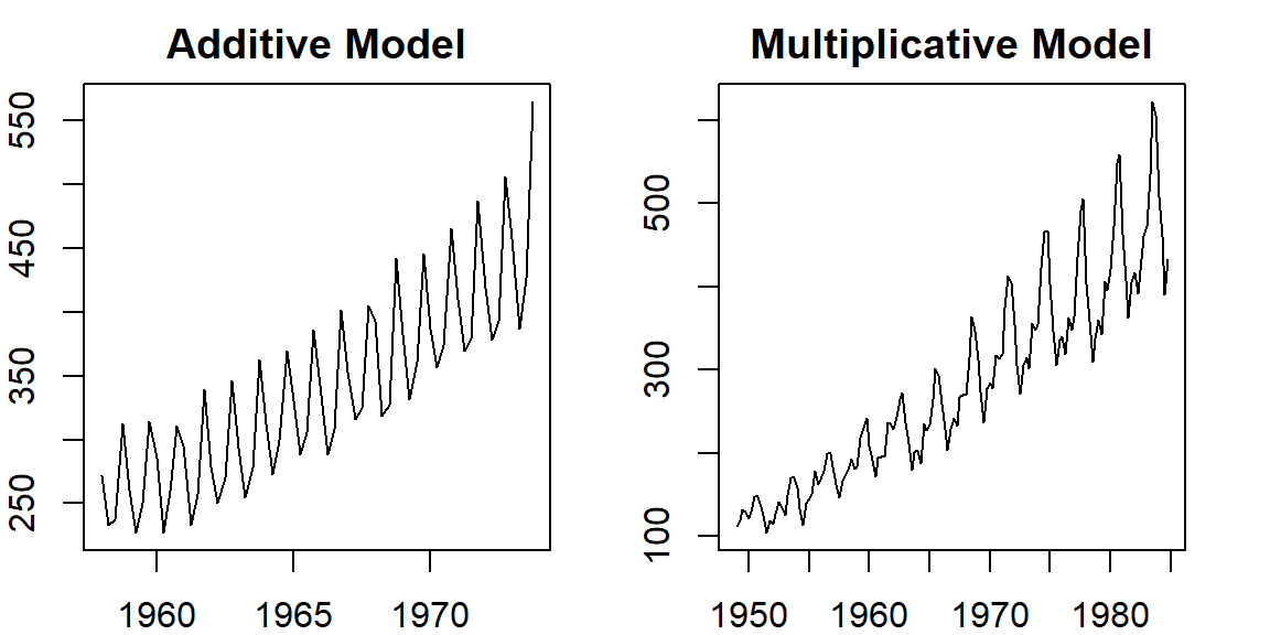
Figure 15.1: time series plots of additive and multiplicative series
Denote \(T = trend\), \(S = seasonality\), and \(E = error\). With these notations, we can characterize the structure of additive and multiplicative time series.
In a multiplicative time series, the components multiply together to make the time series. As the time series increases in magnitude, the seasonal variation increases as well. The structure of a multiple time series has the following form.
\[ y_t = T_t \times S_t \times E_t. \]
In an additive time series, the components add together to make the time series. If you have an increasing trend, you still see roughly the same size peaks and troughs throughout the time series. This is often seen in indexed time series where the absolute value is growing but changes stay relative. The structure of an additive time series has the following form
\[ y_t = T_t + S_t + E_t. \]
For an additive time series, the detrended additive series has for \(D_t = y_t - T_t\). For the multiplicative time series, the detrended time series is calculated by \(D_t = y_t/T_t\)
15.2 Understanding the Classical Decomposition of Time Series
To understand the structure of additive and multiplication ties series, we decompose these time series by calculating the trend, seasonality, and errors manually by writing a basic R script to gain a technical understanding of decomposing a time series. At the very end of this section, we introduce the R function decompose() to extract the three components of additive and multiplicative time series.
15.2.1 Detect Trend
To detect the underlying trend, we use a smoothing technique called moving average and it’s variant centered moving average. For a seasonal time series, the width of the moving window must be the same as the seasonality. Therefore, to decompose a time series we need to know the seasonality period: weekly, monthly, etc.
Example 1: Australian beer production data has an annual seasonality. Since the data set is quarterly data, the moving average window should be 4.
trend.beer = ma(ausbeer.ts, order = 4, centre = T)  # centre = T => centered moving average
par(mar=c(2,2,2,2))
plot(as.ts(ausbeer.ts), xlab="", ylab="", col="darkred", lwd =2)
title(main = "Extract trend from Australia Beer Production")
lines(trend.beer, lwd =2, col = "blue")
legend("topleft", c("original series", "trend curve"), lwd=rep(2,2),
       col=c("darkred", "blue"), bty="n")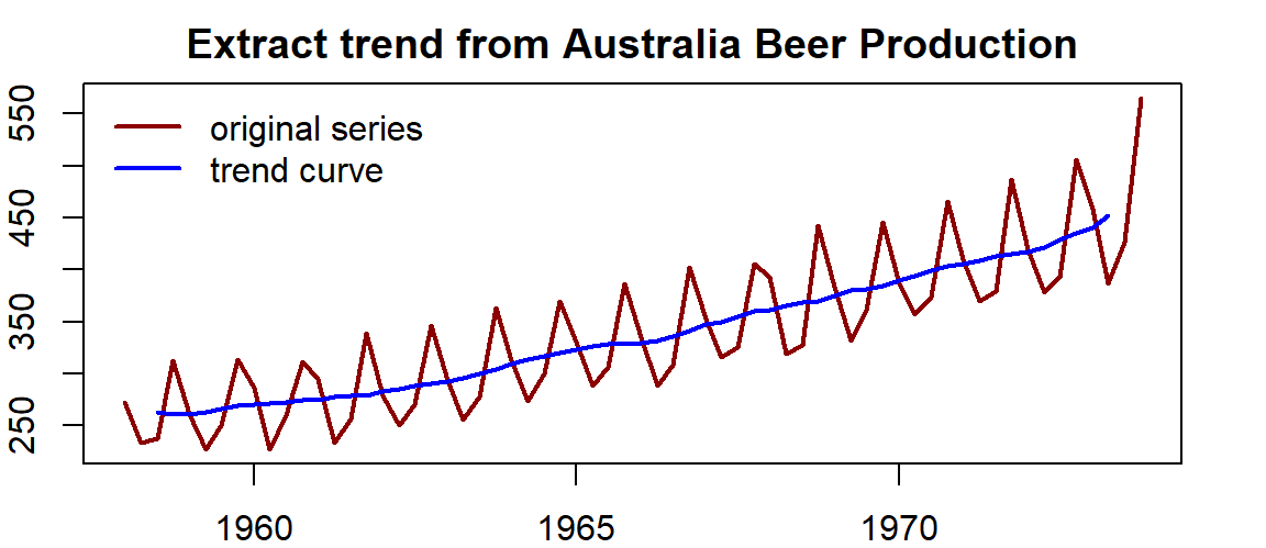
Figure 15.2: Serires plot with trend curve
Example 2: The airline passenger data were recorded monthly. It has an annual seasonal pattern. We choose a moving average window of 12 to extract the trend from this multiplicative time series.
trend.air = ma(AirPassengers.ts, order = 12, centre = T)  # centre = T => centered moving average
par(mar=c(2,2,2,2))
plot(as.ts(AirPassengers.ts), xlab="", ylab="", col="darkred", lwd =2)
title(main = "Extract trend from Airline Passengers Monthly Data")
lines(trend.air, lwd =2, col = "blue")
legend("topleft", c("original series", "trend curve"), lwd=rep(2,2),
       col=c("darkred", "blue"), bty="n")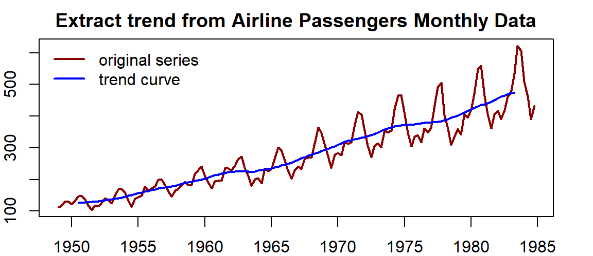
Figure 15.3: series plot with curve trend
The moving averages of both time series are recorded in the above two code chunks and will be used to restore the original series.
The process of removing the trend from a time series is called detrending time series.
The way of detrending a time series is dependent on the types of the time series. The following code shows how to calculate the detrended time series.
Example 3: We calculate the detrended series using the Australian Beer data and the Airline Passengers data as an example.
detrend.beer = ausbeer.ts - trend.beer
detrend.air = AirPassengers.ts/trend.air
par(mar=c(2,2,2,2))
par(mfrow=c(1,2))
# plot(ausbeer.ts, xlab="", main = "Australia Beer", col="darkred")
# plot(AirPassengers.ts, xlab="", main = "Air Passengers", col="blue")
plot(detrend.beer, xlab="", main = "Australia Beer", col="darkred")
plot(detrend.air, xlab="", main = "Air Passengers", col="blue")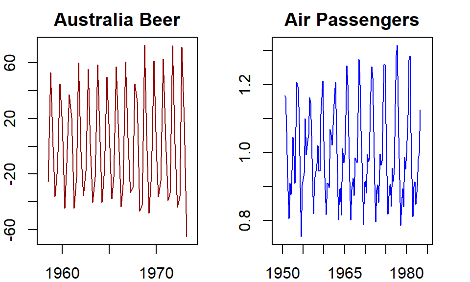
Figure 15.4: Detrended series
The technique we used in removing the trend from a time series model is a non-parametric smoothing procedure. There are different techniques in statistics to estimate a curve for a given set. The moving average is one of the simplest ones and is widely used in time series.
15.2.2 Extracting the Seasonality
Similar to the trend in a time series, the seasonality of a time series is also a non-random structural pattern. We can extract the seasonality from the detrended time series.
The idea is to redefine a seasonal series based on the detrended series by replacing all observations taken from the same seasonal period with the average of these observations. This process is called averaging seasonality. This idea is implemented in R. Here is how to do it in R.
Example 4: Use the Australian Beer Production Data and the Airline Passenger Data after their trends were removed. The following code illustrates how to calculate and graph the seasonality of both series.
par(mfrow=c(2,1), mar=c(3,2,3,2))
## Australia Beer
mtrx.beer = t(matrix(data = detrend.beer, nrow = 4))
seasonal.beer = colMeans(mtrx.beer, na.rm = T)
seasonal.beer.ts = as.ts(rep(seasonal.beer,16))
plot(seasonal.beer.ts, xlab = "", col="darkred", main="Seasonal series of Australia beer")
##
mtrx.air = t(matrix(data = detrend.air, nrow = 12))
seasonal.air = colMeans(mtrx.air, na.rm = T)
seasonal.air.ts = as.ts(rep(seasonal.air,16))
plot(seasonal.air.ts, xlab = "", col = "blue", main="Seasonal series of air passengers")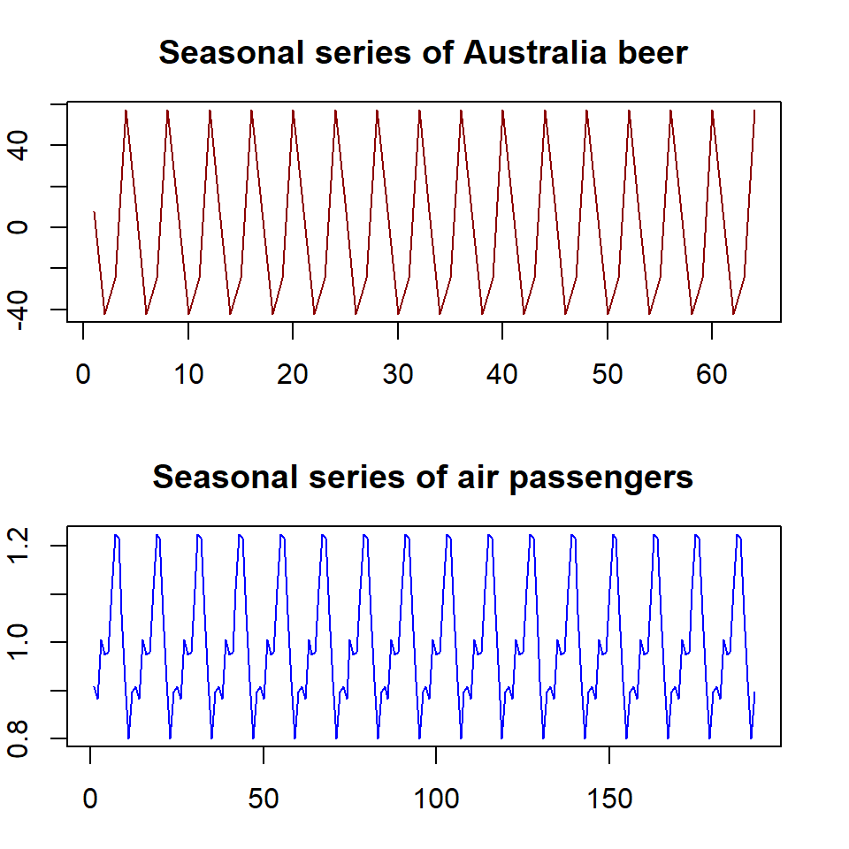
Figure 15.5: Seasonal series
15.2.3 Extracting Remainder Errors
The error term is the random component in the time series. We learned the of extracting the trend and seasonality from the original time series. How to extract the “random” noise from a given time series?
In the additive model, the random error term is given by \(E_t = y_t - T_t -S_t\). The random error for a multiplicative model is given by \(E_t = y_t/(T_t \times S_t)\).
Example 5: Use the above formulas to separate the random error components in additive and multiplicative models using Australian beer production and Airline passenger series data.
random.beer = ausbeer.ts - trend.beer - seasonal.beer
random.air = AirPassengers.ts / (trend.air * seasonal.air)
##
par(mfrow=c(2,1), mar=c(3,2,3,2))
plot(random.beer , xlab = "", col="darkred", main="Random errors of Australia beer")
plot(random.air, xlab = "", col = "blue", main="Random errors of air passengers")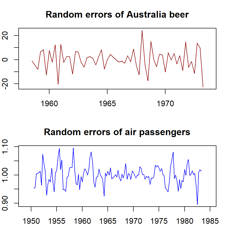
Figure 15.6: Random error components
15.2.4 Reconstruct the Original Series / Compose New Series
The original series can be reconstructed by using the decomposed components. Since the moving average technique was used in the detrending series, the resulting reconstructed series with \(T_t\), \(S_t\), and \(E_t\) will generate a few missing values in the beginning and the end depending on the width of the moving average window.
Example 6: Reconstruct the original series of Australian beer data and the airline passenger data.
recomposed.beer = trend.beer+seasonal.beer+random.beer
recomposed.air = trend.air*seasonal.air*random.air
par(mfrow=c(1,2), mar=c(3,2,3,2))
plot(ausbeer.ts, col="darkred", lty=1)
lines(recomposed.beer, col="blue", lty=2, lwd=2)
legend("topleft", c("original series", "reconstructed series"),
       col=c("darkred", "blue"), lty=1:2, lwd=1:2, cex=0.8, bty="n")
title(main="Australian Beer")
##
plot(AirPassengers.ts, col="darkred", lty=1)
lines(recomposed.air, col="blue", lty=2, lwd=2)
legend("topleft", c("original series", "reconstructed series"),
       col=c("darkred","blue"), lty=1:2, lwd=1:2, cex=0.8, bty="n")
title(main="Airline Passengers")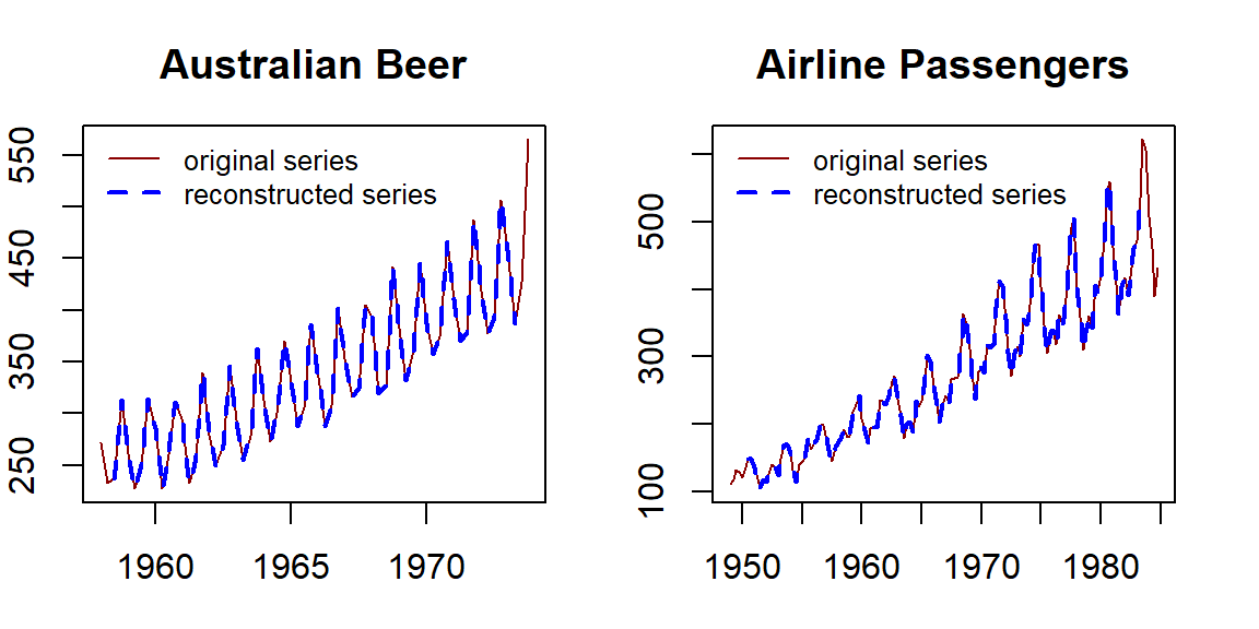
Figure 15.7: Adding trend series to the original series
15.2.5 Decomposing Time Series with decompose()
The R library forecast was created by a team led by a leading expert in the discipline. We’ll use the R function decompose( ) in library{forecast} as a decomposition function to decompose a series into seasonal, trend, and random components. The Australian beer production (additive) and airline passenger numbers (multiplicative) will still be used to illustrate the steps.
Example 6: Plot the components of the Australian beer production data.
decomp.beer = decompose(ausbeer.ts, "additive")
## plot the decomposed components
par(mar=c(2,2,2,2), oma=c(0,2,2,0))
plot(decomp.beer, col="darkred", xlab="")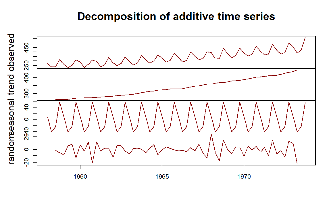
Example 7: Plot the components of the Airline Passenger Data.
decomp.air = decompose(AirPassengers.ts, "multiplicative")
## plot the decomposed components
par(mar=c(2,2,2,2), oma=c(0,2,2,0))
plot(decomp.air, col= "navy", xlab="")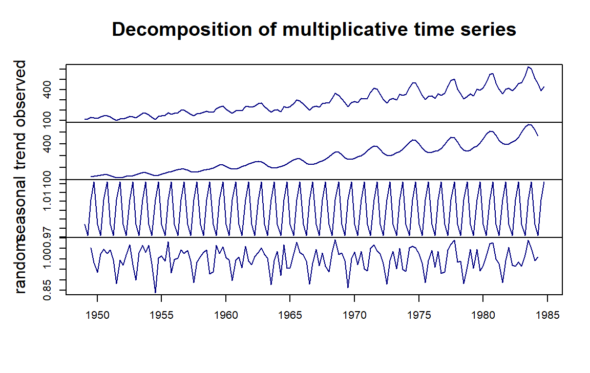
Th R function decompose() can be used to extract the individual components from a given additive and multiplicative model using the following code.
Example 8: Decomposing Australian beer production data using decompose().
decomp.beer = decompose(ausbeer.ts, "additive")
# the four components can be extracted by
seasonal.beer = decomp.beer$seasonal
trend.beer = decomp.beer$trend
error.beer = decomp.beer$random
Example 9: Decomposing airline passengers data using decompose().
decomp.air = decompose(AirPassengers.ts, "multiplicative")
# the four components can be extracted by
seasonal.air = decomp.air$seasonal
trend.air = decomp.air$trend
error.air = decomp.air$random
Concluding Remark: There are other decomposition methods. among them, X11 is commonly used in econometrics. The recently developed method STL() that used LOESS algorithm to estimate the trend can also be used to extract components from more general time series. We will outline this decomposition method to forecast future values.
15.3 Forecasting with Decomposing
Several benchmark forecasting methods were introduced in the previous module. Next, we use these benchmark methods to forecast the deseasonalized series. Since the seasonality of a time series is a scalar, we can forecast the deseasonalized series through decomposition and then adjust the forecasted values.
15.3.1 Forecasting Additive Models with Decomposing
Since the multiplicative models can be converted to an additive model by
\[ \log(y_t) = \log(S_t) + \log(T_t) + \log(E_t). \]
So we only restrict our discussion in this module to additive models. Assuming an additive decomposition, the decomposed time series can be written as
\[y_t = \hat{S}_t + \hat{A}_t\]
where \(\hat{A}_t = \hat{T} + \hat{E}_t\) is the seasonally adjusted component. We can forecast the future values based on \(\hat{A}_t\).
Example 10: Forecasting based on the seasonally adjusted series with Australian beer production data. We introduced four benchmark forecasting methods in the previous module. For a time series with a trend, naive, seasonal naive, and drift method is more accurate than the moving average. The issue is that none of the benchmark methods forecast the trend. As an illustrative example, we use the naive method to forecast the deseasonalized series and then add the seasonal adjustment to the forecast values.
decomp.beer = decompose(ausbeer.ts, "additive")
# the four components can be extracted by
seasonal.beer = decomp.beer$seasonal
trend.beer = decomp.beer$trend
error.beer = decomp.beer$random
seasonal.adj = trend.beer + error.beer
deseasonalized.pred = as.data.frame(rwf(na.omit(seasonal.adj), h = 6))
seasonality =  matrix(rep(seasonal.beer[3:8],5), nco=5, byrow=F)
seasonal.adj.pred <- deseasonalized.pred  + seasonality
kable(seasonal.adj.pred, caption = "Forecasting with decomposing - drift method")| Point Forecast | Lo 80 | Hi 80 | Lo 95 | Hi 95 | |
|---|---|---|---|---|---|
| 1973 Q3 | 404.7167 | 386.3725 | 423.0608 | 376.6617 | 432.7717 |
| 1973 Q4 | 486.6167 | 460.6741 | 512.5593 | 446.9409 | 526.2924 |
| 1974 Q1 | 437.1500 | 405.3769 | 468.9231 | 388.5573 | 485.7427 |
| 1974 Q2 | 387.0000 | 350.3116 | 423.6884 | 330.8900 | 443.1100 |
| 1974 Q3 | 404.7167 | 363.6978 | 445.7355 | 341.9838 | 467.4496 |
| 1974 Q4 | 486.6167 | 441.6828 | 531.5505 | 417.8962 | 555.3371 |
Since the deseasonalized series has two missing values in the beginning and two in the end. we remove the missing values before using the drift methods to forecast the next 6 periods (qtr3, 1973 - qtr 4, 1874). The forecast values are given in the above table.
par(mar=c(2,2,2,2))
plot(1:62, as.vector(ausbeer.ts)[-c(63,64)], type="l", xlim=c(1,70), ylim=c(200, 570),
     xlab="", ylab="Beer Production", main="Forecast with classical decomposing")
lines(62:64,  as.vector(ausbeer.ts)[c(62,63,64)], col="red")
points(62:64,  as.vector(ausbeer.ts)[c(62,63,64)], col="red", pch=21)
lines(63:68,seasonal.adj.pred[,1], col="blue")
points(63:68,seasonal.adj.pred[,1], col="blue", pch = 16)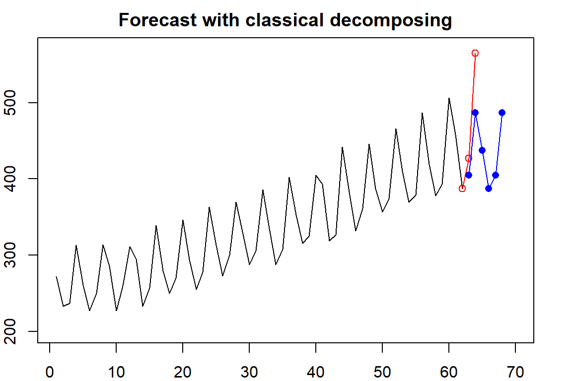
Figure 15.8: forecasting with classical decomposing
The plot of the forecast values and the original values. The red plot represented quarters 3-4 of 1973 and forecast values in quarters 3 - quarters 4, 1974, are plotted in blue. We can see that
15.3.2 Concepts of Seasonal and Trend Decomposition Using Loess (STL)
Seasonal and Trend decomposition using LOESS (STL) combines the classical time series decomposition and the modern locally estimated scatterplot smoothing (LOESS). The LOESS has developed about 40 years ago and is a modern computational algorithm. The seasonal trend in a time series is a fixed pattern. The real benefit of STL is to use the LOESS to estimate the nonlinear trend more accurately. We will not discuss the technical development of the STL. Instead, we will use its R implementation to decompose time series and use it to forecast future values.
stl.beer = stl(ausbeer.ts, "periodic")
seasonal.stl.beer   <- stl.beer$time.series[,1]
trend.stl.beer     <- stl.beer$time.series[,2]
random.stl.beer  <- stl.beer$time.series[,3]
###
par(mfrow=c(4,1), mar=c(2,2,2,2))
plot(ausbeer.ts)
plot(as.ts(seasonal.stl.beer))
plot(trend.stl.beer)
plot(random.stl.beer)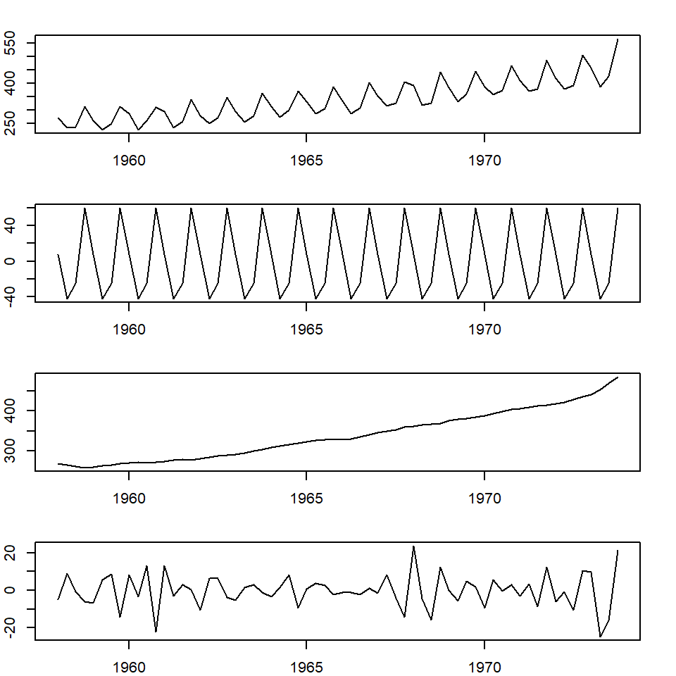
Figure 15.9: Decomposing with STL approach
We can also plot the above-decomposed components in a single step as follows with the STL model.
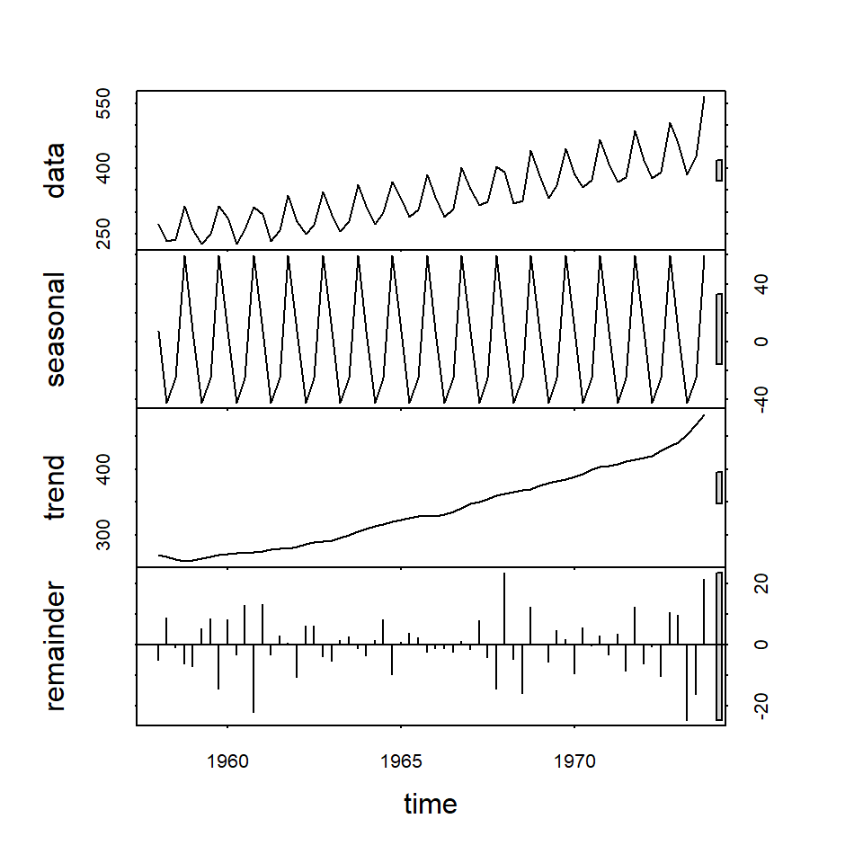
Figure 15.10: plot component panel with STL object
15.3.3 Forecast with STL decomposing
For the additive model, we can use the R function stl() to decompose the series into three components. It uses a more robust non-parametric smoothing method (LOESS) to estimate the nonlinear trend.
fit <- stl(ausbeer.ts,s.window="periodic")
par(mar=c(2,2,2,2))
plot(forecast(fit,h=6, method="rwdrift"))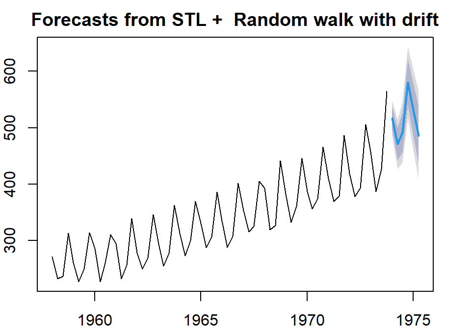
Figure 15.11: Forecas with STL decomposing
15.3.4 Length of Time Series
The length of the time series impacts the performance of the forecasting. In general, a very long time series (for example, more than 200 observations) usually does not work well for most of the existing models partly because the existing models were not built for very long series. Intuitively, future values are dependent on recent historical values. If including too old observations that have no predictive power in the model will bring bias and noise to the underlying model and, hence, negative impacts on the performance of the model.
There are a lot of discussions in literature and practice about the minimum size required for building a good time series model. It seems that 60 is the suggested minimum size. The actual minimum size depends on the situation and the level of accuracy.
In this class, we recommend the sample size be between 60 and 200. Therefore, in the assignment, if the original time series data has more than 200 observations, we can use only 150-200 most recent data values for analysis.
15.4 Case Study
15.4.1 Data description and
The time series used in this case study is chosen from https://datahub.io/search: 10-year nominal yields on US government bonds from the Federal Reserve. The 10-year government bond yield is considered a standard indicator of long-term interest rates. The data contains monthly rates. There are 808 months of data between April 1943 and July 2020. We only use look at monthly data between January 2008 and July 2020.
15.4.2 Define time series object
Since this is monthly data, frequency =12 will be used the define the time series object.
usbond.ts = ts(data.us.bond[,2], frequency = 12, start = c(2008, 1))
par(mar=c(2,2,2,2))
plot(usbond.ts, main="US Bond Rates Between Jan, 2008 and July, 2020", ylab="Monthly Rate", xlab="")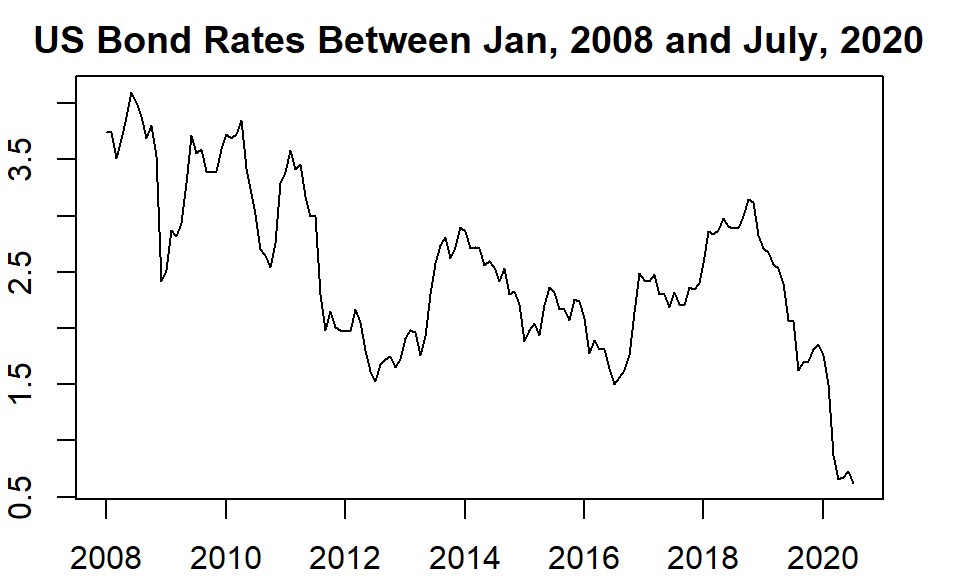
Figure 15.12: US bond monthly rates
15.4.3 Forecasting with Decomposing
Notice that the classical decomposition method does not work as well as the STL method due to the robustness of the LOESS component. The following visual representations show the different behaviors of the two methods of decomposition.
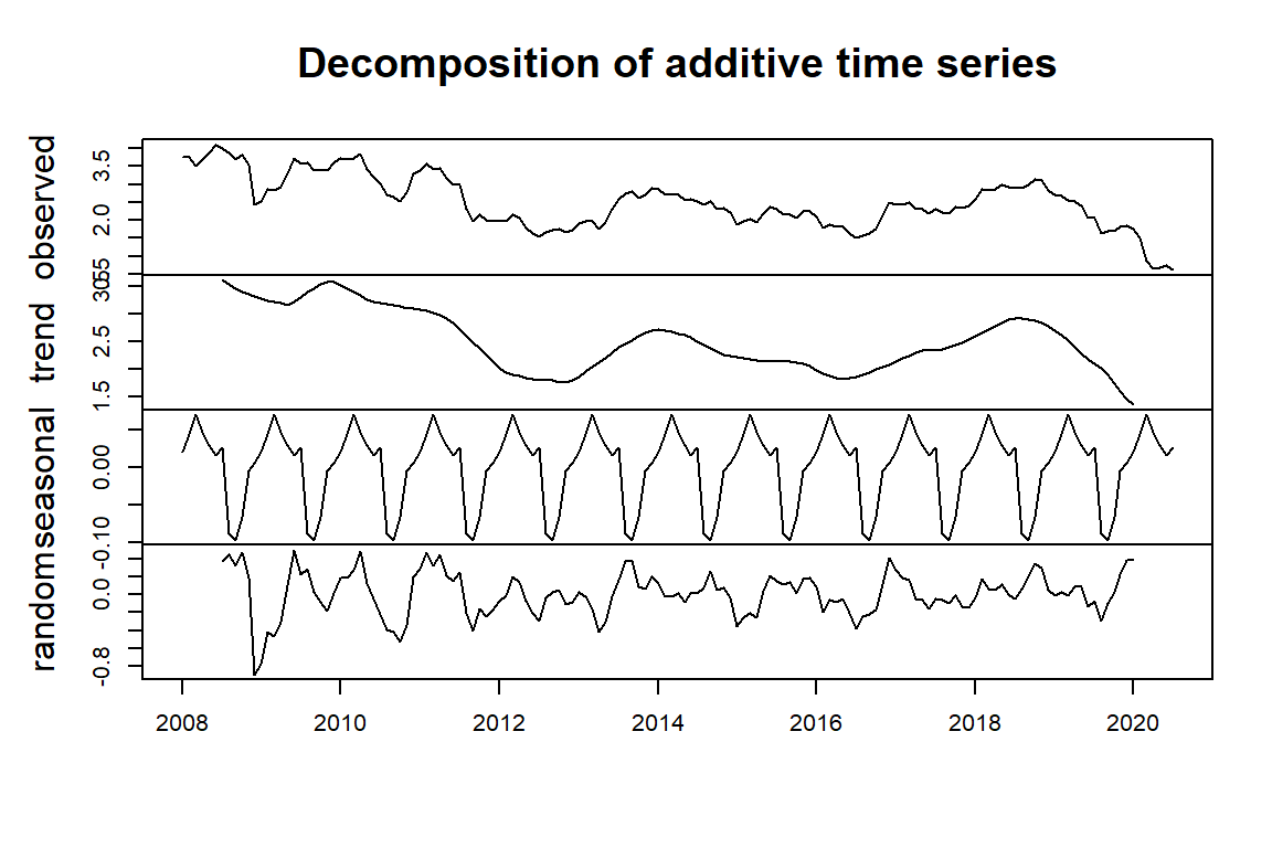
Figure 15.13: Classical decomposition of additive time series
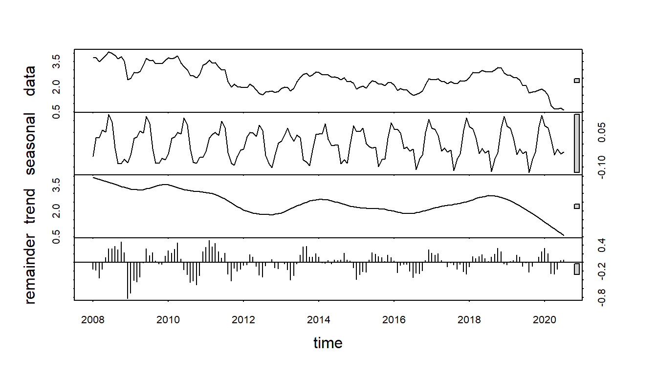
Figure 15.14: STL decomposition of additive time series
Training and Testing Data
We hold up the last 7 periods of data for testing. The rest of the historical data will be used to train the forecast model.
To evaluate the effect of different sizes in training the time series, We define different training data sets with different sizes. Three training set sizes used in this example are 144, 109, 73, and 48. The same test set with size 7 will be used to calculate the prediction error.
ini.data = data.us.bond[,2]
n0 = length(ini.data)
##
train.data01 = data.us.bond[1:(n0-7), 2]
train.data02 = data.us.bond[37:(n0-7), 2]
train.data03 = data.us.bond[73:(n0-7), 2]
train.data04 = data.us.bond[97:(n0-7), 2]
## last 7 observations
test.data = data.us.bond[(n0-6):n0,2]
##
train01.ts = ts(train.data01, frequency = 12, start = c(2008, 1))
train02.ts = ts(train.data02, frequency = 12, start = c(2011, 1))
train03.ts = ts(train.data03, frequency = 12, start = c(2014, 1))
train04.ts = ts(train.data04, frequency = 12, start = c(2016, 1))
##
stl01 = stl(train01.ts, s.window = 12)
stl02 = stl(train02.ts, s.window = 12)
stl03 = stl(train03.ts, s.window = 12)
stl04 = stl(train04.ts, s.window = 12)
## Forecast with decomposing
fcst01 = forecast(stl01,h=7, method="naive")
fcst02 = forecast(stl02,h=7, method="naive")
fcst03 = forecast(stl03,h=7, method="naive")
fcst04 = forecast(stl04,h=7, method="naive")
We next perform error analysis.
## To compare different errors, we will not use the percentage for MAPE
PE01=(test.data-fcst01$mean)/fcst01$mean
PE02=(test.data-fcst02$mean)/fcst02$mean
PE03=(test.data-fcst03$mean)/fcst03$mean
PE04=(test.data-fcst04$mean)/fcst04$mean
###
MAPE1 = mean(abs(PE01))
MAPE2 = mean(abs(PE02))
MAPE3 = mean(abs(PE03))
MAPE4 = mean(abs(PE04))
###
E1=test.data-fcst01$mean
E2=test.data-fcst02$mean
E3=test.data-fcst03$mean
E4=test.data-fcst04$mean
##
MSE1=mean(E1^2)
MSE2=mean(E2^2)
MSE3=mean(E3^2)
MSE4=mean(E4^2)
###
MSE=c(MSE1, MSE2, MSE3, MSE4)
MAPE=c(MAPE1, MAPE2, MAPE3, MAPE4)
accuracy=cbind(MSE=MSE, MAPE=MAPE)
row.names(accuracy)=c("n.144", "n.109", "n. 73", "n. 48")
kable(accuracy, caption="Error comparison between forecast results with different sample sizes")| MSE | MAPE | |
|---|---|---|
| n.144 | 0.7967685 | 0.4518108 |
| n.109 | 0.7718715 | 0.4463052 |
| n. 73 | 0.7665760 | 0.4449924 |
| n. 48 | 0.8055530 | 0.4649921 |
plot(1:4, MSE, type="b", col="darkred", ylab="Error", xlab="",
     ylim=c(0.4,.85),xlim = c(0.5,4.5), main="Error Curves", axes=FALSE)
labs=c("n=144", "n=109", "n=73", "n=48")
axis(1, at=1:4, label=labs, pos=0.4)
axis(2)
lines(1:4, MAPE, type="b", col="blue")
text(1:4, MAPE+0.03, as.character(round(MAPE,4)), col="blue", cex=0.7)
text(1:4, MSE-0.03, as.character(round(MSE,4)), col="darkred", cex=0.7)
legend(1.5, 0.63, c("MSE", "MAPE"), col=c("darkred","blue"), lty=1, bty="n", cex=0.7)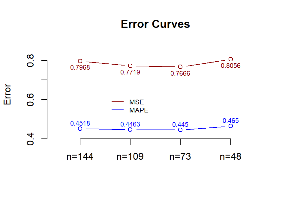
Figure 15.15: Comparing forecast errors
We trained the same algorithm with different sample sizes and compared the resulting accuracy measures. Among four training sizes 144, 109, 73, and 48. training data size 73 yields the best performance.
As anticipated, forecasting with STL smoothing does not yield decent results. However, our case study still accomplishes the main learning goals. To be more specific, we have learned how to
decompose a time series
distinguish the graphical patterns of additive and multiplicative time series models
use the non-parametric smoothing LOESS method in time series forecasting;
use the technique of machine learning to tune the training size to identify the optimal training size to achieve the best accuracy. In this case, the training size is considered a tuning parameter (hyper-parameter).
We will start building actual and practical forecasting models in the next module - exponential smoothing models.
15.5 Analysis Assignment
This assignment focuses on the conceptual understanding of decomposing time series and forecasting with decomposing. As mentioned in the closing paragraph of the case study in the class note, the goals of this assignment are (1) to enhance your conceptual understanding of methods of decomposition and forecasting; (2) to find the appropriate training size to produce the best performance.
The following websites contain some time series data. You can find one time series that has at least 150 observations. If your data set has more than 150, you choose 150-200 most recent observations to complete the assignment. The analysis and components in the analysis should be similar to that in the case study in the class note.
You can also find your data set from other sites for this assignment.