Topic 3 Base R Graphical Functions
This note introduces the graphical capabilities of base R graphical functions. Base R graphical system contains a set of high-level plotting functions such as plot(), hist(), barplot(), etc., and also a set of low-level functions that are used jointly with the high-level plotting functions such as points(), lines(), text(), segments(), etc. to make a flexible graphical system.
3.1 R Graphic Devices
R is able to output graphics to the screen or save them directly to a file (e.g. postscript, pdf, svg, png, jpeg, etc.). The different functions for producing graphical output are known as Graphic Devices. For example, pdf() would invoke the pdf device, while png() would invoke the png device. Type ?Devices into the R console to see a list of graphical devices that are available to R on your system.
By default, graphical output is sent to the screen. As R is cross-platform, the graphics device for producing **screen*“** graphics differs by the system. The available fonts may also differ by the system and graphical device.
3.2 Plotting with Base Graphics: plot()
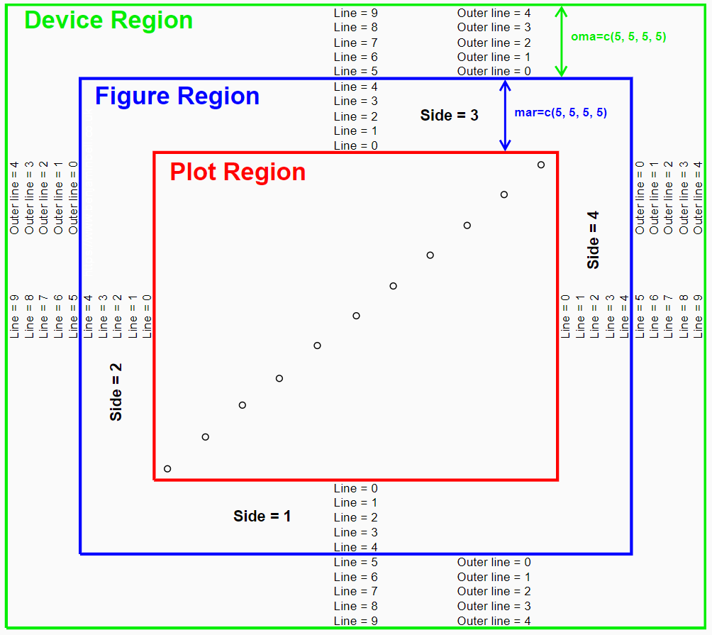
plot() is the most important high-level graphic function. When using plot(), the output is sent to the graphics device. This creates a “plot region” on the graphics device. The visible area of the graphics device is also known as the “device region”. The plot region on the other hand is the area of the plot (usually bounded by a box) and does not include the plot axes, labels, or margins.
The plot region, plus the axes, labels, and margins are known as the “figure region”. Often, the device region and figure region can be the same size - but they are not the same thing.
3.2.1 Outer and Inner Margins
par(mar=c(x, x, x, x), oma = c(x, x, x, x))
Almost all kinds of plots, charts, and graphs can be produced using base graphics, These plots can be fully customized using par() (graphical parameter). The following figure explains the graphical parameters we can use to customize the graphical layout.
Example 1: We make a scatter plot of the two numerical variable in the well-known data set iris. To make nearly overlapped data points distinguishable, we are going to use R function alpha() in the library scales.
We read the data from the GitHub repository.
library(knitr)
library(scales)
iris = read.table("https://raw.githubusercontent.com/pengdsci/sta321/main/ww02/w02-iris.txt", header = TRUE)
par(mfrow = c(1,1), oma=c(1, 1, 1, 1), mar=c(2, 2, 2, 2))
plot(iris$SepalLength, iris$PetalLength, pch = 16, cex = 1.5)
title(main="Sepal Length vs Petal Length (Outer)",
      outer=TRUE,
      col.main = "red",
      cex.main=1)
title(main="Sepal Length vs Petal Length (Inner)",
      outer=FALSE,
      col.main = "blue",
      cex.main=0.8)
## Coloring points with the transparency level
## species ID
setosa = which(iris$Classification == "Iris-setosa")
versicolor = which(iris$Classification == "Iris-versicolor")
virginica = which(iris$Classification == "Iris-virginica")
## adding points
points(iris$SepalLength[setosa], iris$PetalLength[setosa],
       pch=16,
       col = alpha("purple", 0.5),    # add a transparency level
       cex = 1.5)
points(iris$SepalLength[versicolor], iris$PetalLength[versicolor],
       pch=16,
       col = alpha("blue", 0.5),
       cex = 1.5)
points(iris$SepalLength[virginica], iris$PetalLength[virginica],
       pch=16,
       col = alpha("red", 0.5),
       cex = 1.5)
legend("bottomright", c("setosa", "versicolor", "virginica"),
       col=c("purple", "blue", "red"),
       pch=rep(16,3), cex=rep(1.5,3), bty="n")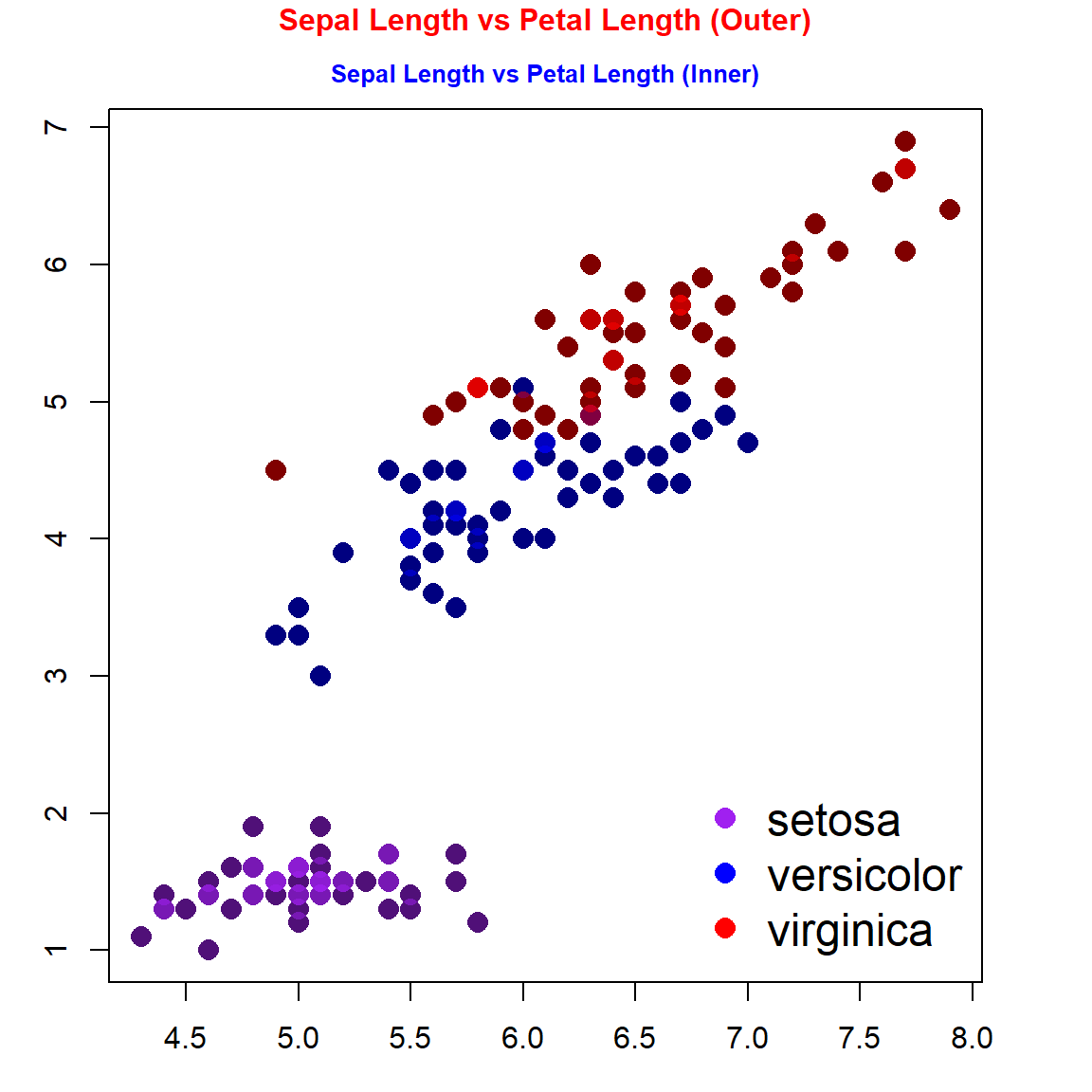
3.2.2 Simple multi-panel Plots
layout() or par(mfrow = c())
Example 2
iris = read.table("https://raw.githubusercontent.com/pengdsci/sta321/main/ww02/w02-iris.txt", header = TRUE)
## species ID
setosa = which(iris$Classification == "Iris-setosa")
versicolor = which(iris$Classification == "Iris-versicolor")
virginica = which(iris$Classification == "Iris-virginica")
###
par(mfrow = c(1,2), oma=c(2, 2, 2, 2), mar=c(2, 2, 2, 2))
plot(iris$SepalLength, iris$PetalLength, pch = 16, cex = 1.5,
            xlab = "Sepal Width",
            ylab = "Petal Width")
title(main="Sepal Length vs Petal Length",
      outer=FALSE,
      col.main = "blue",
      cex.main=0.8)
## adding points
points(iris$SepalLength[setosa], iris$PetalLength[setosa],
       pch=16,
       col = alpha("purple", 0.5),
       cex = 1.5)
points(iris$SepalLength[versicolor], iris$PetalLength[versicolor],
       pch=16,
       col = alpha("blue", 0.5),
       cex = 1.5)
points(iris$SepalLength[virginica], iris$PetalLength[virginica],
       pch=16,
       col = alpha("red", 0.5),
       cex = 1.5)
legend("bottomright", c("setosa", "versicolor", "virginica"),
       col=c("purple", "blue", "red"),
       pch=rep(16,3), cex=0.8, bty="n")
##
plot(iris$SepalWidth, iris$PetalWidth, pch = 16, cex = 1.5,
            xlab = "Sepal Width",
            ylab = "Petal Width")
title(main="Sepal Length vs Petal Length",
      outer=FALSE,
      col.main = "blue",
      cex.main=0.8)
## adding points
points(iris$SepalWidth[setosa], iris$PetalWidth[setosa],
       pch=16,
       col = alpha("purple", 0.5),
       cex = 1.5)
points(iris$SepalWidth[versicolor], iris$PetalWidth[versicolor],
       pch=16,
       col = alpha("blue", 0.5),
       cex = 1.5)
points(iris$SepalWidth[virginica], iris$PetalWidth[virginica],
       pch=16,
       col = alpha("red", 0.5),
       cex = 1.5)
legend("right", c("setosa", "versicolor", "virginica"),
       col=c("purple", "blue", "red"),
       pch=rep(16,3), cex=0.8, bty="n")
## Overall Title
title(main="Comaring Sepal and Petal Sizes",
      outer=TRUE,
      col.main = "darkred",
      cex.main=1.2)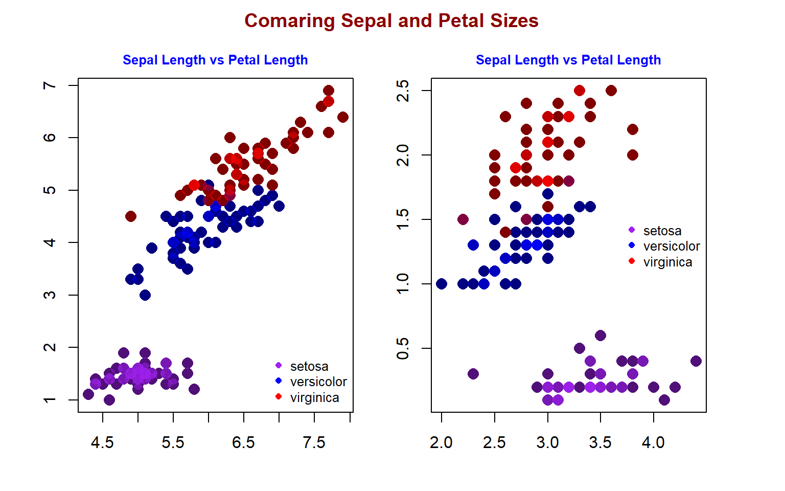
3.3 Making Our Own Colors
We can make transparent colors using R and the rgb() command. These colors can be useful for charts and graphics with overlapping elements.
The rgb() command defines a new color using numerical values (0–255) for red, green and blue. In addition, we also set an alpha value (also 0–255), which sets the transparency (0 being fully transparent and 255 being “solid”).
The following example takes the standard blue and makes it transparent (~50%):
mycol <- rgb(0, 0, 255, max = 255, alpha = 125, names = "blue50")
You can also use col2rgb() to check the composition of an existing named R color and modify it to define your own favorite colors.
Example 3: We check the RGB code from several named R colors in the following
##       [,1]
## red    139
## green    0
## blue 0## [,1]
## red 135
## green 206
## blue 235## [,1]
## red 255
## green 215
## blue 0## [,1]
## red 160
## green 32
## blue 240Example 3 We define a color by modifying “gold” and “purple”. I take the average of the RGB codes of “gold” and “purple” to see what the color looks like.
ratio = 0.4
avggoldpurple = round(ratio*col2rgb("gold") + (1-ratio)*col2rgb("purple"))
##
mycol.1 = rgb(avggoldpurple[1,1], avggoldpurple[2,1], avggoldpurple[3,1], max = 255, alpha = 125, names = "goldpuple50")
###
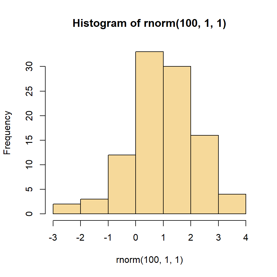
hist(rnorm(100),  col = mycol.1)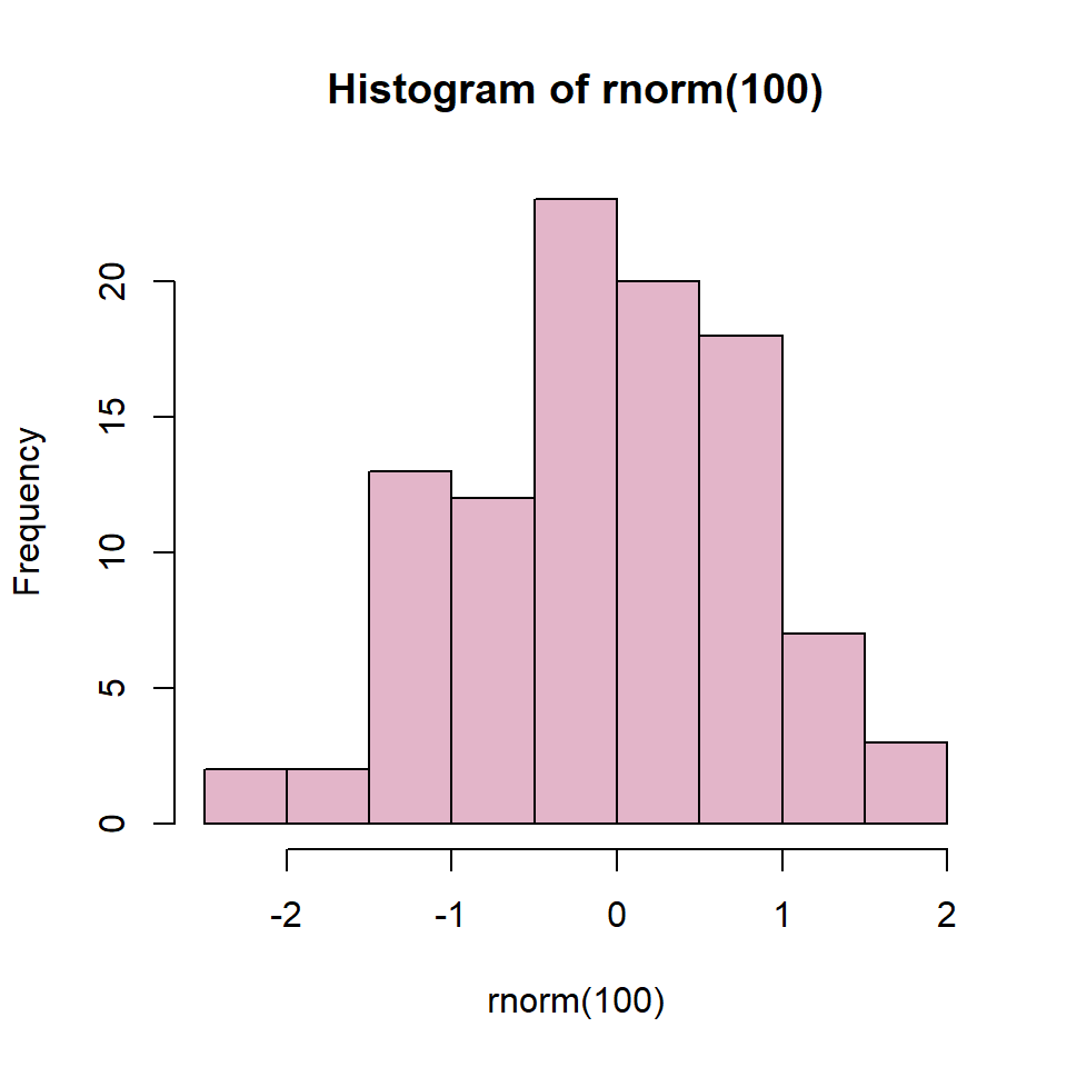
ratio = 0.8
avggoldpurple = round(ratio*col2rgb("gold") + (1-ratio)*col2rgb("purple"))
##
mycol.2 = rgb(avggoldpurple[1,1], avggoldpurple[2,1], avggoldpurple[3,1], max = 255, alpha = 125, names = "goldpuple50")
###
hist(rnorm(100,1,1),  col = mycol.2)