Topic 2 R, RStudio and RMarkdown
This chapter introduces open-source free computation and technical writing tools for this course: R, RStudio, and RMarkdown.
2.1 R
R is a programming language and free software environment for statistical computing and graphics supported by the R Foundation for Statistical Computing. The R language is widely used among statisticians and data miners for developing statistical software and data analysis. – Wikipedia
The official R web page has download links: https://www.r-project.org/. You can download and install the most current version of R based on your machine’s operating system.
2.1.1 Order of Operations
The order of basic operations that we will use in this class is given below.
PEMDAS: Parentheses => Exponential => Multiplication => Division => Addition => Subtraction!
When calculating confidence intervals and test statistics based on given formulas, please keep PEMDAS in mind!
(2+7)/(3^2)*5-1 = 9/9*5-1 = 5 - 1 = 4We check the answer directly by typing the following in the R Console:
## [1] 42.1.2 Basic R Objects
We introduce several basic R objects (or R data structures): vectors, matrices, lists, and data frames.
R is case-sensitive, so name and Name will refer to different objects!
Name <- 1
name <- 0
2.1.2.1 Vectors
- An R vector holds a set of numerical values or character strings. For example,
## [1] 1.0000000 4.0000000 2.1000000 1.6094379 3.1415927 0.9092974 0.6065307 0.0000000## [1] "john" "david" "jones" "kate"Note A single scalar is considered a vector (i.e., one-dimensional vector).
2.1.2.2 Matrices
An R matrix is a rectangular table that holds either numerical or character values, but not both types of values. The following are two examples.
##           [,1]      [,2]
## [1,] 1.0000000 4.0000000
## [2,] 2.1000000 1.6094379
## [3,] 3.1415927 0.9092974
## [4,] 0.6065307 0.0000000## [,1] [,2]
## [1,] "john" "jones"
## [2,] "david" "kate"Note that the values in vectors and matrices must be in the same data type. A scalar is also considered as a 1-by-1 matrix.
2.1.2.3 Lists
A list is an R structure that may contain objects of any other type, including other lists. Lots of the modeling functions produce lists as their return values. We define a list to hold vectors and matrices defined in the previous sub-sections.
## $numvec
## [1] 1.0000000 4.0000000 2.1000000 1.6094379 3.1415927 0.9092974 0.6065307 0.0000000
##
## $charvec
## [1] "john" "david" "jones" "kate"
##
## $nummtx
## [,1] [,2]
## [1,] 1.0000000 4.0000000
## [2,] 2.1000000 1.6094379
## [3,] 3.1415927 0.9092974
## [4,] 0.6065307 0.0000000
##
## $charmtx
##      [,1]    [,2]
## [1,] "john"  "jones"
## [2,] "david" "kate"The following example shows how to access the objects in an R list.
##           [,1]      [,2]
## [1,] 1.0000000 4.0000000
## [2,] 2.1000000 1.6094379
## [3,] 3.1415927 0.9092974
## [4,] 0.6065307 0.0000000
2.1.2.4 Data Frame
A data frame is a table or a two-dimensional array-like structure in which each column contains values of one variable and each row contains one set of values from each column.
The following are the characteristics of a data frame.
The column names should be non-empty.
The row names should be unique.
The data stored in a data frame can be of numeric, factor, or character type.
Each column should contain the same number of data items.
The following is an example of a data frame
# Create the data frame.
emp.data <- data.frame(
   emp.id = c (1:5),
   emp.name = c("Rick","Dan","Michelle","Ryan","Gary"),
   salary = c(623.3,515.2,611.0,729.0,843.25),

   start_date = as.Date(c("2012-01-01", "2013-09-23", "2014-11-15", "2014-05-11",
      "2015-03-27"))
)
# Print the data frame.
print(emp.data)
## emp.id emp.name salary start_date
## 1 1 Rick 623.30 2012-01-01
## 2 2 Dan 515.20 2013-09-23
## 3 3 Michelle 611.00 2014-11-15
## 4 4 Ryan 729.00 2014-05-11
## 5 5 Gary 843.25 2015-03-272.2 RStudio
RStudio is a must-know tool for everyone who works with the R programming language. It’s used in data analysis to import, access, transform, explore, plot, model data, and make predictions on data.
2.2.1 RStudio GUI
The RStudio interface consists of several windows. I insert an image of a regular RStudio GUI.
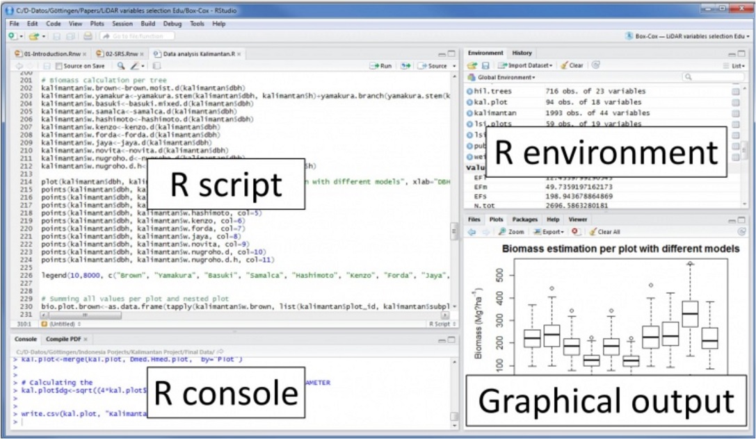
Figure 2.1: List of all variables and the description of each variable
2.2.2 Console
We can type commands directly into the console, or write in a text file, and then send the command to the console. It is convenient to use the console if your task involves one line of code. Otherwise, we should always use an editor to write code and then run the code in the Console.
2.2.3 Source Editor
Generally, we will want to write programs longer than a few lines. The Source Editor can help you open, edit, and execute these programs.
2.2.4 Environment Window
The Environment window shows the objects (i.e., data frames, arrays, values, and functions) in the environment (workspace). We can see the descriptive information such as the types and dimensions of the objects in your environment. We also choose data sources from the environment to view in the source window like a spreadsheet.
2.2.5 System and Graphic files
The Files tab has a navigable file manager, just like the file system on your operating system. The Plot tab is where the graphics you create will appear. The Packages tab shows you the packages that are installed and those that can be installed (more on this just now). The Help tab allows you to search the R documentation for help and is where the help appears when you ask for it from the Console.
2.2.6 RStudio offers numerous helpful features:
- A user-friendly interface
- The ability to write and save reusable scripts
- Easy access to all the imported data and created objects (like variables, functions, etc.)
- Exhaustive help on any object
- Code autocompletion
- The ability to create projects to organize and share your work with your collaborators more efficiently
- Plot previewing
- Easy switching between terminal and console
After you install R on your machine, you can go to https://posit.co/products/open-source/rstudio/ to download the free version of RStudio and install it. R will be automatically connected to RStudio. You can then open the Markdown through the GUI of RStudio.
2.3 RMarkdown
An R Markdown document is a text-based file format that allows you to include descriptive text, code blocks, and code output. It can be converted to other types of files such as PDF, HTML, and WORD that can include code, plots, and outputs generated from the code chunks.
2.3.1 Code Chunk
In R Markdown, we can embed R code in the code chunk defined by the symbol ```{} and closed by ```. The symbol `, also called backquote or backtick, can be found on the top left corner of the standard keyboard as shown in the following.
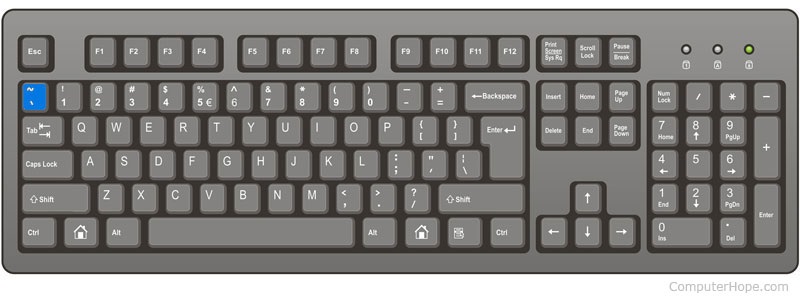
Figure 2.2: The location of backquote on the standard keyboard
There are two code chunks: executable and non-executable chunks. The following code chunk is non-executable since there is no argument specified in the {}.
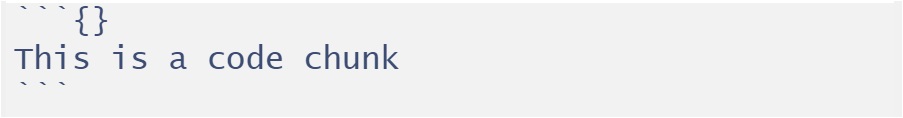
Figure 2.3: Non-executable code chunk.
This is a code chunkTo write a code chunk that will be executed, we can simply put the letter r inside the curly bracket. If the code the code chunk is executable, you will the green arrow on the top-right corner of the chunk.
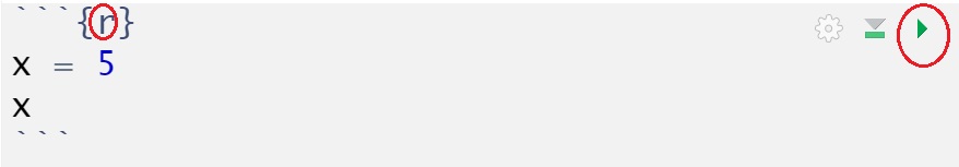
Figure 2.4: Executable code chunk.
We can define R objects with and without any outputs. In the above R code chunk, we define an R object under the name x and assign the value 5 to x (the first line of the code). We also request an output that prints the value of x. The above executable code chunk gives output [1] 5 in the Markdown document. The same output in the knit output files is in a box with a transparent background in the form ## [1] 5.
## [1] 5We can also use an argument in the code chunk to control the output. For example, the following code chunk will be evaluated when kitting to other formats of files. But we can still click the green arrow inside the code chunk to evaluate the code.
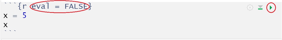
Figure 2.5: Executable code chunk with control options.
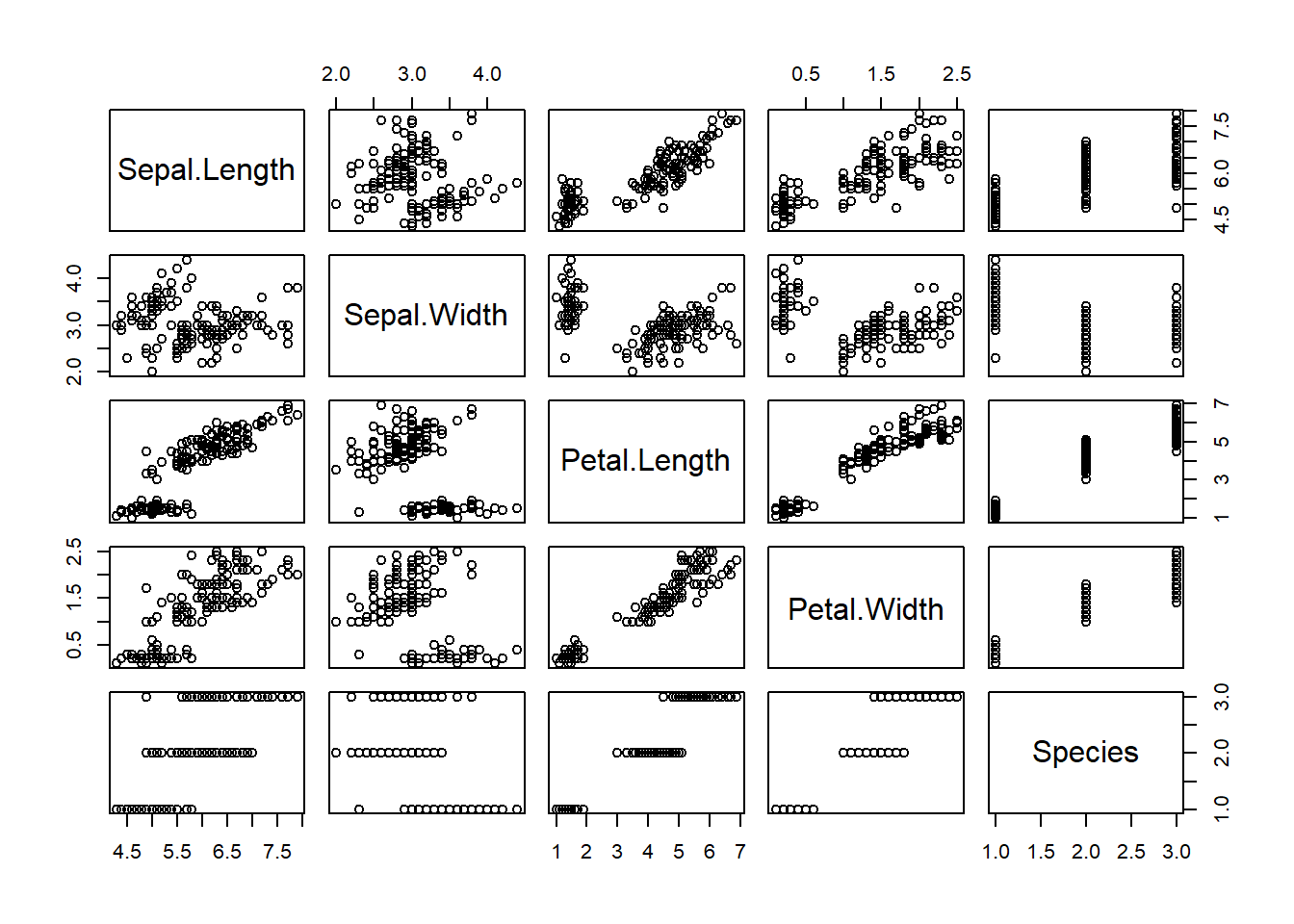
2.3.2 Graphics Generated from R Code Chunks
In the previous sub-sections, we include images from external image files. In fact, can use the R function to generate graphics (other than interacting with plots, etc.) in the markdown file & knit. For instance, we can generate the following image from R and include it in the Markdown document and the knitter output files.