Topic 12 Logistic Regression Models
Linear regression models are used to assess the association between the continuous response variable and other predictor variables. If the response variable is a binary categorical variable, the linear regression model is not appropriate. We need a new model, the logistic regression model, to assess the association between the binary response variable and other predictor variables.
This module focuses on the regression model with a binary response.
12.1 Motivational Example and Practical Question
Example : Longevity in male fruit flies is positively associated with adult size. However, reproduction has a high physiological cost that could impact longevity.
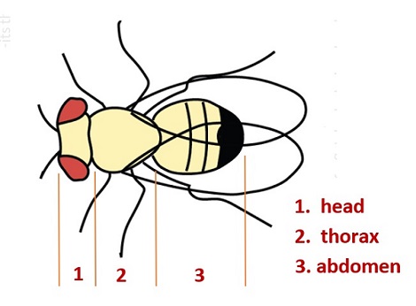
The original study looks at the association between longevity and adult size in male fruit flies kept under one of two conditions. One group is kept with sexually active females over the male’s life span. The other group is cared for in the same way but kept with females who are not sexually active.
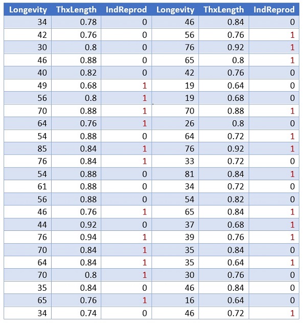
Figure 12.1: Fruit Flies Data Table
The above table gives the longevity in days for the male fruit flies allowed to reproduce (IndReprod = 0) and for those deprived of the opportunity (IndReprod = 1).
The data was collected from a case-control study design. The original study association analysis using the multiple linear regression model in which Longevity was a response variable and Thorax and IndReprod were used as predictor variables. In this example, we build a logistic regression to assess the association between longevity and reduction. Due to the case-control study design, the resulting logistic regression cannot be used as a predictive model.
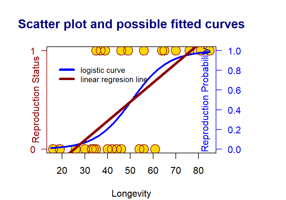
Figure 12.2: The scatter plots of a binary response v.s. a continuous predictor variable
Since the response variable is binary (i.e., it can only take on two distinct values, 0 and 1 in this example), the linear regression line is a bad choice since (1) the response variable is not continuous, (2) the fitted regression line can take on any values between negative infinity and positive infinity. The response variable takes on only either 0 or 1 (see the dark red straight line).
A meaningful approach to assess the association between the binary response variable and the predictor variable by looking at how the predictor variables impact the probability of observing the bigger value (i.e., the one that has a higher alphabetical order) of the response variable. The above S curve describes the relationship between the values of the predictor variable(s) and the probability of observing the bigger value of the response variable.
12.2 Logistic Regression Models and Applications
Logistic regression is a member of the generalized linear regression (GLM) family which includes linear regression models. The modeling-building process is the same as that in linear regression modeling.
12.2.1 The Structure of Logistic Regression Model
The actual probability function of observing the bigger value of the response variable for giving the predictor variable is given by
\[ P(Y=1) = \frac{\exp(\beta_0 + \beta_1 \text{Longevity})}{1 + \exp(\beta_0 + \beta_1 \text{Longevity})} \]
If \(\beta_1\) (also called slope parameter) is equal to zero, the longevity and the reproduction status are NOT associated. Otherwise, there is an association between the response and the predictor variables. The sign of the slope parameter reflects the positive or negative association.
12.2.2 Assumptions and Diagnostics
There are assumptions for the binary logistic regression model.
The response variable must be binary (taking on only two distinct values).
Predictor variables are assumed to be uncorrelated.
The functional form of the predictor variables is correctly specified.
The model diagnostics for logistic regression are much more complicated than in the linear regression models. We will not discuss this topic in this course.
12.2.3 Coefficient Estimation and Interpretation
The estimation of the logistic regression coefficients is not as intuitive as we saw in the linear regression model (regression lines and regression plane or surface). An advanced mathematical method needs to be used to estimate the regression coefficient. The R function glm() can be used to find the estimate of regression coefficients.
The interpretation of the coefficients of the logistic regression model is also not straightforward. In the motivational example, the value of \(\beta_1\) is the change of log odds of observing reproduction status to be 1. As usual, we will not make an inference of the intercept. In case-control data, the intercept is inestimable.
The output of glm() contains information similar to what has been seen in the output of lm() in the linear regression model.
12.2.4 Use of glm() and Annotations
We use the motivational example to illustrate the setup of glm() and the interpretation of the output.
## Fit the logistic regression
mymodel =glm(IndReprod ~ Longevity,   # model formula (response on the left).
          family=binomial,            # must be binomial for the binary response!
          data=fruitflies)            # data frame name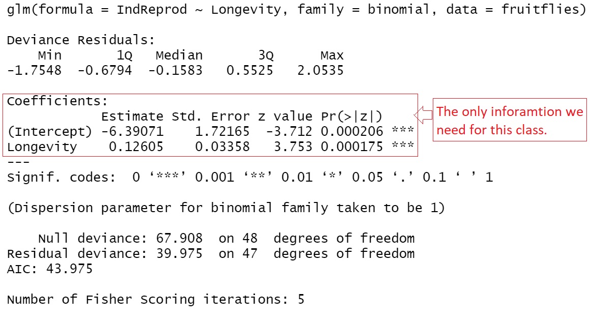
Figure 12.3: The complete output of glm()
The output has four major pieces of information: the model formula, the five-number-summary of the deviance residuals, significant test results of the predictor variables, and goodness-of-fit measures. In this course, we only focus on the significance tests.
12.2.5 Applications of Logistic Regression Models
Like other regression models, the logistic regression models have two basic applications: association analysis and prediction analysis.
The association analysis focuses on the interpretation of the regression coefficients that have information about whether predictor variables are associated with the response variable through the probability of the bigger value of the response variable.
Since the logistic regression builds the relationship between the probability of observing the bigger value of the response and the predictor variable, predicting the value of the response variable requires a cut-off probability to assign a value of 1 or 0 to the response variable. The prediction process of a logistic regression model is depicted in the following figure.
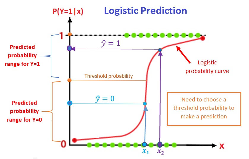
Figure 12.4: Prediction process of the logistic regression models
12.3 Case Studies
We present two examples in this section.
12.3.1 The simple logistic regression model
Suzuki et al. (2006) measured sand grain size on 28 beaches in Japan and observed the presence or absence of the burrowing wolf spider Lycosa ishikariana on each beach. Sand grain size is a measurement variable, and spider presence or absence is a nominal variable. Spider presence or absence is the dependent variable; if there is a relationship between the two variables, it would be sand grain size affecting spiders, not the presence of spiders affecting the sand.
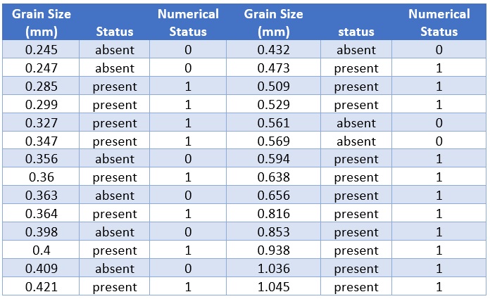
Figure 12.5: Spider Data Table
grainsize=c(0.245, 0.247, 0.285, 0.299, 0.327, 0.347, 0.356, 0.360, 0.363, 0.364,
            0.398, 0.400, 0.409, 0.421, 0.432, 0.473, 0.509, 0.529, 0.561, 0.569,
            0.594, 0.638, 0.656, 0.816, 0.853, 0.938, 1.036, 1.045)
status=c(0, 0, 1, 1, 1, 1, 0, 1, 0, 1, 0, 1, 0, 1, 0, 1, 1, 1, 0, 0, 1, 1, 1, 1,
         1, 1, 1, 1)
spider = as.data.frame(cbind(grainsize = grainsize, status = status))
Fitting a Simple Logistic Regression Model
Since there is only one predictor variable in this study, simply choose the simple linear regression model to this data set.
spider.model = glm(status ~ grainsize,
                   family = binomial,
                   data = spider)
significant.tests = summary(spider.model)$coef
pander(significant.tests, caption = "Summary of the significant tests of
the logistic regression model")| Estimate | Std. Error | z value | Pr(>|z|) | |
|---|---|---|---|---|
| (Intercept) | -1.648 | 1.354 | -1.217 | 0.2237 |
| grainsize | 5.122 | 3.006 | 1.704 | 0.08844 |
Association Analysis
The above significant tests indicate that the grain size does not achieve significance (p-value = 0.08844) at level 0.05. Note that the p-value is calculated based on the sample, it is also a random variable. Moreover, the sample size in this study is relatively small. We will claim the association between the two variables. As the grain size increases by one unit, the log odds of observing the wolf spider burrowing increase by 5.121553. In other words, the grain size and the presence of spiders are positively associated.
Prediction Analysis
As an example, we choose two new grain sizes 0.33 and 0.57, and want to predict the presence of the wide spiders on the beaches with the given grain sizes. We used the R function predict() in linear regression, we used the same function to predict the logistic regression model.
spider.model = glm(status ~ grainsize,
                   family = binomial,
                   data = spider)
##
mynewdata = data.frame(grainsize=c(0.275, 0.57))
pred.prob = predict(spider.model, newdata = mynewdata,
        type = "response")
## threshold probability
cut.off.prob = 0.5
pred.response = ifelse(pred.prob > cut.off.prob, 1, 0)  # predicts the response
pred.table = cbind(new.grain.size = c(0.275, 0.57),
                   pred.response = pred.response)
pander(pred.table, caption = "Predicted Value of response variable
with the given cut-off probability")| new.grain.size | pred.response |
|---|---|
| 0.275 | 0 |
| 0.57 | 1 |
12.3.2 Multiple Logistic Regression Model
In this case study, we used a published study on bird introduction in New Zealand. The objective is to predict the success of avian introduction to New Zealand. Detailed information about the study can be found in the following article. https://stat501.s3.amazonaws.com/w11-Correlates-of-introduction-success-in-exotic.pdf. The data is included in the article. A text format data file was created and can be downloaded or read directly from the following URL: https://stat501.s3.amazonaws.com/w11-birds-data.txt.
 The response variable: Status - status of success
Predictor variables:
The response variable: Status - status of success
Predictor variables:
- length - female body length (mm)
- mass = female body mass (g)
- range = geographic range (% area of Australia)
- migr = migration score: 1= sedentary, 2 = sedentary and migratory, 3 = migratory
- insect = the number of months in a year with insects in the diet
- diet = diet score: 1 = herbivorous; 2 = omnivorous, 3 = carnivorous.
- clutch = clutch size
- broods = number of broods per season
- wood = use as woodland scored as frequent(1) or infrequent(2)
- upland = use of the upland as frequent(1) or infrequent(2)
- water = use of water scored as frequent(1) or infrequent(2)
- release = minimum number of release events
- indiv = minimum of the number of individuals introduced.
We next read the data from the given URL directly to R. Since there are some records with missing values. We drop those records with at least one missing value.
There are several categorical variables with numerical codings. Among them, migr and diet have three categories and the rest of the categorical variables have two categories. In practice, a categorical variable with more than two categories must be specified as factor variables so R can define dummy variables to capture the difference across the difference.
We conducted an exploratory analysis on nigr and diet and found a flat discrepancy across the effect.We simply treat them as a discrete numerical variable using the numerical coding as the values of the variables.
birds = "https://raw.githubusercontent.com/pengdsci/STA501/main/Data/w11-birds-data.txt"
NZbirds=read.table(birds, header=TRUE)
birds = na.omit(NZbirds)- Build an Initial Model
We first build a logistic regression model that contains all predictor variables in the data set. This model is usually called the full model. Note that the response variable is the success status (1 = success, 0 = failure). Species is a kind of ID, it should not be included in the model.
initial.model = glm(status ~ length + mass + range + migr + insect + diet +
                      clutch + broods + wood + upland + water + release + indiv,
                    family = binomial, data = birds)
coefficient.table = summary(initial.model)$coef
pander(coefficient.table, caption = "Significance tests of logistic regression model")| Estimate | Std. Error | z value | Pr(>|z|) | |
|---|---|---|---|---|
| (Intercept) | -6.338 | 5.717 | -1.109 | 0.2676 |
| length | -0.002815 | 0.005317 | -0.5294 | 0.5965 |
| mass | 0.002668 | 0.001674 | 1.594 | 0.111 |
| range | -0.1316 | 0.3502 | -0.3758 | 0.7071 |
| migr | -2.044 | 1.116 | -1.831 | 0.06704 |
| insect | 0.148 | 0.2124 | 0.6969 | 0.4859 |
| diet | 2.029 | 1.883 | 1.077 | 0.2814 |
| clutch | 0.07938 | 0.2683 | 0.2959 | 0.7673 |
| broods | 0.02177 | 0.9283 | 0.02345 | 0.9813 |
| wood | 2.49 | 1.642 | 1.517 | 0.1293 |
| upland | -4.713 | 2.865 | -1.645 | 0.09991 |
| water | 0.2349 | 2.67 | 0.08799 | 0.9299 |
| release | -0.01292 | 0.1932 | -0.06685 | 0.9467 |
| indiv | 0.01593 | 0.008324 | 1.913 | 0.05571 |
The p-values in the above significance test table are all bigger than 0.5. We next search for the best model by dropping some of the insignificant predictor variables. Since there are so many different ways to drop variables, next we use an automatic variable procedure to search the final model.
- Automatic Variable Selection
R has an automatic variable selection function step() for searching the final model. We will start from the initial model and drop insignificant variables using AIC as an inclusion/exclusion criterion.
In practice, sometimes, there may be some practically important predictor variables. Practitioners want to include these practically important variables in the model regardless of their statistical significance. Therefore, we can fit the smallest model that includes only those practically important variables. The final model should be between the smallest model, which we will call a reduced model, and the initial model, which we will call a full model. For illustration, we assume insect and range are practically important, we want to include these two variables in the final model regardless of their statistical significance.
In summary, we define two models: the full model and the reduced model. The final best model will be the model between the full and reduced models. The summary table of significant tests is given below.
full.model = initial.model  # the *biggest model* that includes all predictor variables
reduced.model = glm(status ~ range + insect , family = binomial, data = birds)
final.model =  step(full.model,
                    scope=list(lower=formula(reduced.model),upper=formula(full.model)),
                    data = birds,
                    direction = "backward",
                    trace = 0)   # trace = 0: suppress the detailed selection process
final.model.coef = summary(final.model)$coef
pander(final.model.coef , caption = "Summary table of significant tests")| Estimate | Std. Error | z value | Pr(>|z|) | |
|---|---|---|---|---|
| (Intercept) | -3.438 | 2.138 | -1.608 | 0.1079 |
| mass | 0.001939 | 0.0007326 | 2.647 | 0.008119 |
| range | 0.00001412 | 0.3098 | 0.00004558 | 1 |
| migr | -2.024 | 0.9603 | -2.108 | 0.03506 |
| insect | 0.2705 | 0.1426 | 1.897 | 0.05785 |
| wood | 1.949 | 1.317 | 1.479 | 0.139 |
| upland | -4.731 | 2.098 | -2.255 | 0.02415 |
| indiv | 0.01381 | 0.004058 | 3.404 | 0.0006648 |
- Interpretation - Association Analysis
The summary table contains the two practically important variables range and insect. range does not achieve statistical significance (p-value \(\approx\) 1) and insect is slightly higher than the significance level 0.005. Both variables are seemingly positively associated with the response variable.
The following interpretation of the individual predictor variable assumes that other life-history variables and introduction effort variables.
migr and upland are negatively associated with the response variable. The odds of success of introducing migratory birds are lower than the sedentary birds. Similarly, birds using upland infrequently have lower odds of being successfully introduced than those using upland frequently.
insect is significant (p-value =0.058). The odds of success increase as the number of months of having insects in diet increases.
mass and indiv are positively associated with the response variable. The odds of success increase and the body mass increases Similarly, the odds of success increase as the number of minimum birds of the species increases.
wood does not achieve statistical significance but seems to be positively associated with the response variable.
- Predictive Analysis
As an illustration, we use the final model to predict the status of successful introduction based on the new values of the predictor variables associated with two species. See the numerical feature given in the code chunk.
mynewdata = data.frame(mass=c(560, 921),
                       range = c(0.75, 1.2),
                       migr = c(2,1),
                       insect = c(6, 12),
                       wood = c(1,1),
                       upland = c(0,1),
                       indiv = c(123, 571))
pred.cuccess.prob = predict(final.model, newdata = mynewdata, type="response")
##
## threshold probability
cut.off.prob = 0.5
pred.response = ifelse(pred.cuccess.prob > cut.off.prob, 1, 0)# predicts response
## add the new predicted response to Mynewdata
mynewdata$Pred.Response = pred.response
##
pander(mynewdata, caption = "Predicted Value of response variable
with the given cut-off probability")| mass | range | migr | insect | wood | upland | indiv | Pred.Response |
|---|---|---|---|---|---|---|---|
| 560 | 0.75 | 2 | 6 | 1 | 0 | 123 | 0 |
| 921 | 1.2 | 1 | 12 | 1 | 1 | 571 | 1 |
The predicted status of the successful introduction of the two species is attached to the two new data records.
12.4 Practice Problems
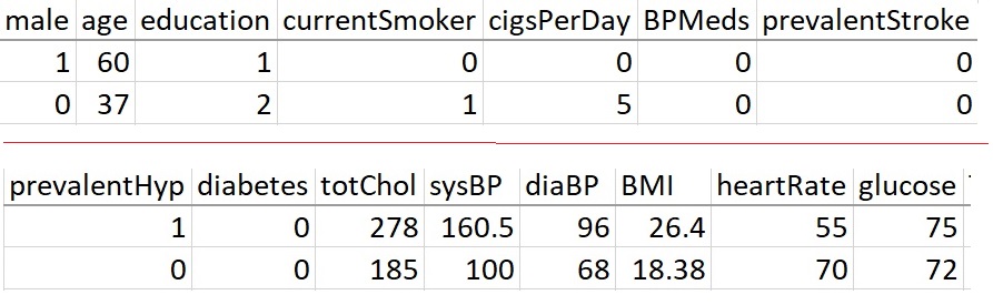
Framingham Heart Study (FHS), a long-term research project developed to identify risk factors of cardiovascular disease, the findings of which had far-reaching impacts on medicine. Indeed, much common knowledge about heart disease—including the effects of smoking, diet, and exercise—can be traced to the Framingham study. The study’s findings further emphasized the need for preventing, detecting, and treating risk factors of cardiovascular disease in their earliest stages
The dataset is a rather small subset of possible FHS datasets, having 4240 observations and 16 variables. The variables are as follows:
- sex : the gender of the observations. The variable is a binary named “male” in the dataset.
- age : Age at the time of medical examination in years.
- education : A categorical variable of the participants’ education, with the levels: Some high school (1), high school/GED (2), some college/vocational school (3), college (4) - caution: This is a numerically coded categorical variable, we need to use the form of factor(education) in the model formulas.
- currentSmoker: Current cigarette smoking at the time of examinations
- cigsPerDay: Number of cigarettes smoked each day
- BPmeds: Use of Anti-hypertensive medication at exam
- prevalentStroke: Prevalent Stroke (0 = free of disease)
- prevalentHyp: Prevalent Hypertensive. The subject was defined as hypertensive if treated
- diabetes: Diabetic according to criteria of the first exam treated
- totChol: Total cholesterol (mg/dL)
- sysBP: Systolic Blood Pressure (mmHg)
- diaBP: Diastolic blood pressure (mmHg)
- BMI: Body Mass Index, weight (kg)/height (m)^2
- heartRate: Heart rate (beats/minute)
- glucose: Blood glucose level (mg/dL)
And finally the response variable:
- TenYearCHD: The 10-year risk of coronary heart disease(CHD).
3658 of these 4240 records are complete cases, and the rest have some missing values. The following code chunk will clean the data and only keep the complete records in the final data set.
fhs = "https://raw.githubusercontent.com/pengdsci/STA501/main/Data/w11-FraminghamCHD.csv"
FHS.data = na.omit(read.csv(fhs))
The above FHS.data has 3658 complete records and 16 variables listed above. The goals of this assignment are both association analysis and predictive analysis. To be more specific, you are expected to follow the analysis in Section 4.2 in the class note.
- Use the above FHS.data to fit an initial model that includes all predictor variables.
- BMI and glucose are two clinically important variables. Both variables will be included in the final model. That is, you can define the smallest model using the two important clinical variables.
- Using an automatic variable selection procedure to identify the final model working model.
- Interpret the regression model coefficients. You don’t have to interpret all coefficients. Pick two coefficients associated with categorical and numerical predictor variables, respectively, to interpret.
- Assume there are two incoming patients with the following demographics and clinical characteristics: