STA490-main

6. Basics of Exploratory Data Analysis (EDA)

Topics and Notes

Working Data Sets

a. Data sources, descriptions, and dictionary DATA SITE
b. Code for loading data CLASS NOTE

Exploratory Data Analysis (EDA) and Applications HTML PDF RMD

b. EDA methods and techniques.
c. Commonly used EDA techniques.
d. Applications of EDA.
e. The EDA process

Visual comparisons of density curves.
Basics of relational database and SQL

a. Concepts of relational database PPT
b. Basic SQL clauses TXT
c. Data sets used in the SQL notes: PLOTS.csv SPECIES.csv SURVEYS.csv

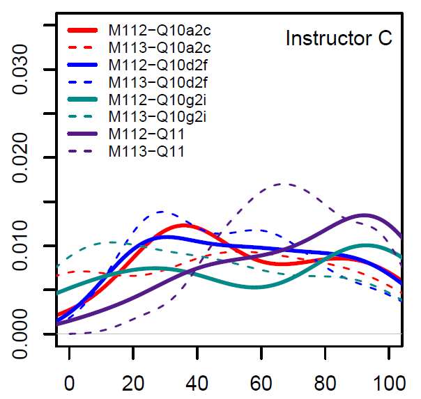
Assignments

Submission Due: Sunday, 11:30 PM.

EDA and Applications with the Combined Bank Loan Data: Please read the

CLASS NOTE

and make sure you fully understand the data set before working on the following assignment items.
1. Delete all records whose MIS_Status value was missing.
2. Change all currency format variables (DisbursementGross, BalanceGross, ChgOffPrinGr, GrAppv, SBA_Appv) to the regular numerical variables (i.e., remove dollar sign and comma separator).
3. Choose any one of the categorical variables in the data set and combine its sparse categories with appropriate categories in a meaningful way so that the refined categorical variable with fewer categories is meaningful and interpretable (Consider the example of course grade, if grade F is a sparse category, the only meaningful way of combining with other category is D). The re-defined categorical variable is suggested to have about 15 or fewer than categories.
4. Calculate the default rates of corresponding categories in the above redefined categorical variable. Note the value CHGOFF of MIS_Status is defined to be loan default. That is, the default rate is the percentage of CHGOFF in MIS_Status.
5. Discretize variable GrAppv into 5 categories (intervals, buckets). This step is equivalent to splitting the original population into 5 subpopulations.
6. Draw the density curves of SBA_Appv for each of the 5 sub-populations defined in 5) and place them on the same plot. The plot should be similar to this overlaid

Density Curves

Go to Table of Contents