Some R Markdown Tips
Cheng Peng
West Chester University
1 More Controls with YAML
One can add some additional controls of the knitted document to the YAML header.
code_folding: "hide"to hide the code chunk to make the knitted document cleaner.code_download: trueto allow downloading RMD source from the HTML page.
3 Commonly Used HTML Tags
Most frequently used HTML tags
<font> </font>- font decoration<a href=""> </a>- hyperlink<img src="">- including an image
<center> </center>-alignment <br>- line breakhr- horizontal line<div>... </div>- divide<p> </p>- paragraph<ul> </ul>- unordered list<ol> </ol>- ordered list<li> </li>- list (<li>) is used with either<ol>or<ul>. The default is<ul>.<table><tr><td> ... </td></tr></table>- defining HTML table<tr>- defining table row<td>- defining table column
| Company | Contact | Country |
|---|---|---|
| Alfreds Futterkiste | Maria Anders | Germany |
| Centro comercial Moctezuma | Francisco Chang | Mexico |
4 Figure in Two Columns
Arguments out.width and out.height apply to
both existing images and R-generated figures.
Unlike the fig.width and fig.height
arguments which only affect dynamic figures, the out.width
and out.height arguments can be used with any type of
graphic and conveniently can accept sizes in pixels or percentages as a
string with % or px as a suffix.
Keep in mind that the % refers to the percent of the HTML container. For example, if the block of text that the image is in is 1000px wide then the image will be 200px using 20%.
out.width can also be used to lay out multi-column
figures.
boxplot(1:10)
plot(rnorm(10))
plot(density(rnorm(100)))


5 Turn Sections to Tabs
Tab format HTML documents are sometimes easy for readers to read the document. R Markdown can convert section-format documents to tab-format documents easily. The following is a simple example based on the popular R mtcars dataset.
5.1 An Example of Tab Format Document
5.1.1 Scatter Plot
As an example, the following scatter plot shows the relationship
between gross horsepower and
mile per gallon.
mtcars %>%
ggplot(aes(x = hp, y = mpg)) +
geom_point()
5.1.2 Summary Table
The following summarized table gives the distributional information of the data set.
summary(mtcars) mpg cyl disp hp
Min. :10.40 Min. :4.000 Min. : 71.1 Min. : 52.0
1st Qu.:15.43 1st Qu.:4.000 1st Qu.:120.8 1st Qu.: 96.5
Median :19.20 Median :6.000 Median :196.3 Median :123.0
Mean :20.09 Mean :6.188 Mean :230.7 Mean :146.7
3rd Qu.:22.80 3rd Qu.:8.000 3rd Qu.:326.0 3rd Qu.:180.0
Max. :33.90 Max. :8.000 Max. :472.0 Max. :335.0
drat wt qsec vs
Min. :2.760 Min. :1.513 Min. :14.50 Min. :0.0000
1st Qu.:3.080 1st Qu.:2.581 1st Qu.:16.89 1st Qu.:0.0000
Median :3.695 Median :3.325 Median :17.71 Median :0.0000
Mean :3.597 Mean :3.217 Mean :17.85 Mean :0.4375
3rd Qu.:3.920 3rd Qu.:3.610 3rd Qu.:18.90 3rd Qu.:1.0000
Max. :4.930 Max. :5.424 Max. :22.90 Max. :1.0000
am gear carb
Min. :0.0000 Min. :3.000 Min. :1.000
1st Qu.:0.0000 1st Qu.:3.000 1st Qu.:2.000
Median :0.0000 Median :4.000 Median :2.000
Mean :0.4062 Mean :3.688 Mean :2.812
3rd Qu.:1.0000 3rd Qu.:4.000 3rd Qu.:4.000
Max. :1.0000 Max. :5.000 Max. :8.000 6 GIF Animation
R has several animation libraries one can use to generate animated graphs to explain some of the complex concepts visually. Sometimes people can generate a series of related images and then use software programs to make a GIF image. This external GIF can also be included in the R Markdown document.
for (i in 1:5) {
pie(c(i %% 5, 1, 3), col = c('red', 'yellow', "blue"), labels = paste(i))
}
7 Load An External image
In addition to the R-generated graphics, we can also include external
images in different formats in the R Markdown document.
out.width= and out.height= options should be
used to control the size of the images.
include_graphics("https://editor.analyticsvidhya.com/uploads/75819stats_1050x520.png")
8 Inline Chunk Options
If too many chunk options are required to lay out the figure, it is not convenient to put all of them in the code chunk. One way to handle this situation is to use inline chunk options.
plot_ly(x=mtcars$wt,y=mtcars$mpg,mode = "markers",color = as.factor(mtcars$vs))My caption
9 Including CSS
There are three ways of inserting a style sheet in the RMarkdown document: inline CSS, internal CSS, and external CSS. We have used all three different formats of CSS in this RMD to format the text or decorate the layout on different occasions. To summarize,
inline CSS: This is an example showing how to change the font size, face, color, etc.
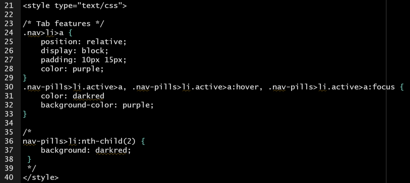
internal CSS: The internal CSS was included at YAML and setup code chunk (Here Is the screenshot)
External CSS: The external CSS style file used in this document can be found (here)
10 Verbatim Code Chunks
Typically we write code chunks and inline expressions that we want to
be parsed and evaluated by knitr. However, if we are trying
to write a tutorial on using knitr`, we may need to generate a verbatim
code chunk or inline expression that is not parsed by knitr, and we want
to display the content of the chunk header and all related options.
```{r out.width=c('50%', '50%'), fig.show='hold'}
boxplot(1:10)
plot(rnorm(10))
plot(density(rnorm(100)))
```